2 People
2.1 What this chapter is about
Economics is about people. As the Bristol economist Alfred Marshall wrote in the first chapter of the book “Principles of Economics” in 1890, “[…] economics is a study of mankind in the ordinary business of life”. In other words, economics is about the interactions and behaviours of normal people in their day to day life. A good starting point for working with economic data is therefore data about people. This chapter is about how to describe changes in the number of people in a region, about quantifying fertility and about measuring life expectancy.
After reading this chapter you should be able to apply the following concepts.
- Distinguishing between stock and flow variables
- Quantifying fertility trends
- Estimating period life expectancy
2.2 Population stocks and flows
2.2.1 What are flow and stock variables?
Economic variables can be classified as either flow or stock variables. We can illustrate the difference between these two types using a bathtub as in Figure 2.1. The water level in the bathtub at a given point in time is a stock variable. The amount of water that has flown into the tub over a period of time is a flow variable.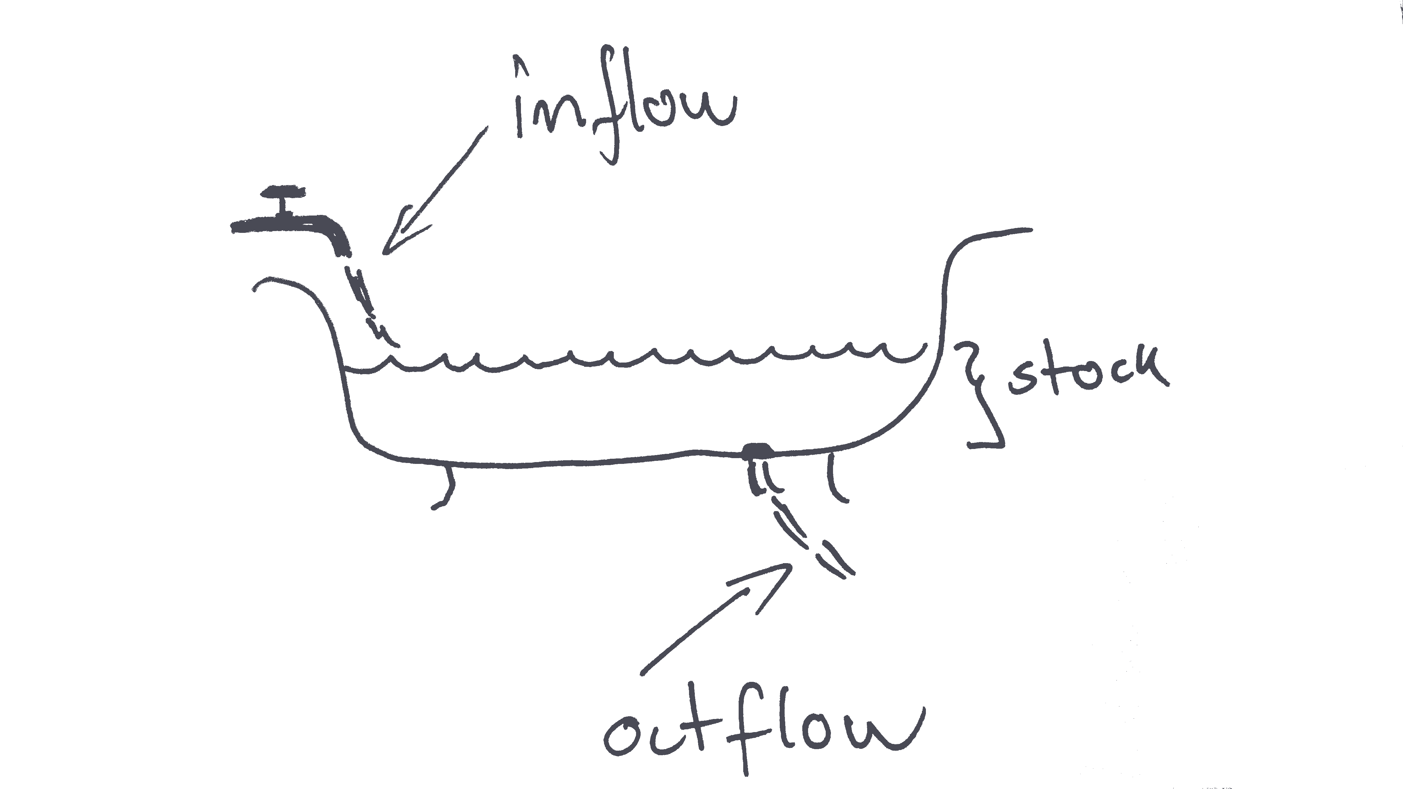
Figure 2.1: A bathtub with water illustrating flows and stocks
An easy way to distinguish between flow and stock variables is that a flow variable is measured over a period of time while a stock variable is measured at a specific point in time.
If someone asked you, “How much water flowed into the bathtub on September 4 at 4:40pm and 10 seconds?”, it would be very difficult to answer because it is difficult to measure the amount of water flowing at a specific second.
However, if someone asked, “How much water was in the bathtub on September 4 at 4:40pm and 10 seconds?”, it would be quite easy to answer (given that you had some tool to measure the level of water). This is because the water level is a stock variable. A stock variable is measured at a point in time and “September 4, at 4:40pm and 10 seconds” is a point in time.
On the other hand if someone asked “How much water flowed into the bathtub between September 4 between 4:40pm and 4:50pm?”, you would also be able to answer it, because you are now given a “period of time” (a period of 10 minutes) which means you are measuring a flow variable.
Let’s think about economic variables instead of water and bathtubs. An example of a stock variable would be wealth. We measure wealth at a “point in time”. For example my wealth at the end of the year. An example of a flow variable would be income. We measure income over a period of time. Can you think of other examples? Is consumption a flow or a stock variable? For example my monthly income.
-
A flow variable measures a flow of quantity over a
period of time.
- For example the flow of migrants into the UK from January 1 2017 to December 31 2017.
-
A stock variable measures the level of quantity at a
point in time.
- For example the number of people residing in the UK on January 1, 2018.
Why is it important to know whether a variable is a flow or stock variable? First, because it is useful if we want to understand changes in a variable over time. The change in the water level of the bathtub (stock) can be described by the inflow (flow) and outflow (flow) of water. The change in wealth (stock) between two points in time depends on the income (flow) and consumption (flow) in the period of time. Second, because the best way to visualize the data depends on the type of variable.
We can often describe the change in a stock variable by underlying flows:
\[ Stock_{1}-Stock_{0}=\Delta Stock=Flow_{0-1} \]
Here we use subscript to denote the point in time (i.e. time 0 and time 1), and the symbol \(\Delta\) to denote changes (it’s the Greek letter “Delta” capitalized). This notation is very common in economics.
For example the change in the population level of the UK from 1 January, 2002 to 1 January, 2003 equals
- the number of people who immigrated to the UK
- minus the number of people who left the UK (emigrated)
- plus the number of children born
- minus the number of people who died
In this example the population level is a stock variable. It is measured at a point in time (January 1, 2002). The other variables are all flow variables that are measured over a period of time. For example the number of births from 1 January 2002 to 1 January, 2003.
We could measure the number of people living in the UK on January 1, 2002 at five seconds and 3 milliseconds after 10:00AM, but how many children are born in exactly that millisecond? A childbirth typically takes more than a second, so how do we allocate a birth a precise millisecond?
2.3 Quantifying fertility trends
We can describe changes in population stocks between two points in time by the underlying population flows. However, we can also dig deeper and get a detailed understanding of changes in population flows. One important reason for changes in population stocks is a change in childbirths. If more children are born, without any changes to the number of people dying or in the number of people migrating, the population stock will increase.
We use a number of specific definitions for descriptions of changes in childbirths over time and differences across regions. Let’s first present these definitions and then discuss data requirements and what the definitions mean.
2.3.1 Definitions
-
Age Specific Fertility Rate (ASFR)
The number of childbirths per woman in a specific age group.
\[\begin{align} ASFR_a=\frac{\text{Number of births to women in age group} a}{\text{Number of women in age group} a} \end{align}\]
-
Total Fertility Rate (TFR):
The number of children born per woman if she were to pass through the childbearing years (typically set to: 15-44y or 15-49y) bearing children according to current age-specific fertility rates.
\[\begin{align} \text{Total Fertility Rate}=\sum_{a=15}^{44}ASFR_a \end{align}\]
-
General Fertility Rate (GFR)
All live births per woman of childbearing ages (also typically per 1000 women).
\[\begin{align} \text{General Fertility Rate}=\frac{\text{Number of births }}{\text{Number of women of childbearing age} } \end{align}\]
Crude Birth Rate (CBR)
All live births per 1000 people of all ages \[\begin{align} CBR=\frac{\text{Number of births }}{\text{Population size} } \end{align}\]
2.3.2 Data requirements
In order to be able to calculate the fertility rates described above we need data on:
- the number of children born by women in specific age groups.
- the number of women in each age group.
- number of people in the population.
Note that 1. above is a flow variable and 2. and 3. are stock variables. When calculating fertility rates we divide a flow variable with a stock variable. It is therefore important to pay attention to the timing of the measurement. Should the population levels (2. and 3.) be measured at the beginning, in the middle, or at the end of the year?
We can obtain such data from statistical agencies such as Eurostat. In Figure 2.2) we show the Total Fertility Rate and General Fertility Rate for the United Kingdom over the last five decades using data from Eurostat. We observe how the two lines representing respectively the General Fertility Rate and the Total Fertility Rate follow each other closely, although they are measured at very different scales. In 1970 a woman in the UK gave birth to on average more than 2.3 children, given the age specific fertility rates in that year. Today that number has dropped to less than 2. There are considerable fluctuations in these rates. The lowest fertility rates were observed around 2000, when the Total Fertility Rate dropped to around 1.8.
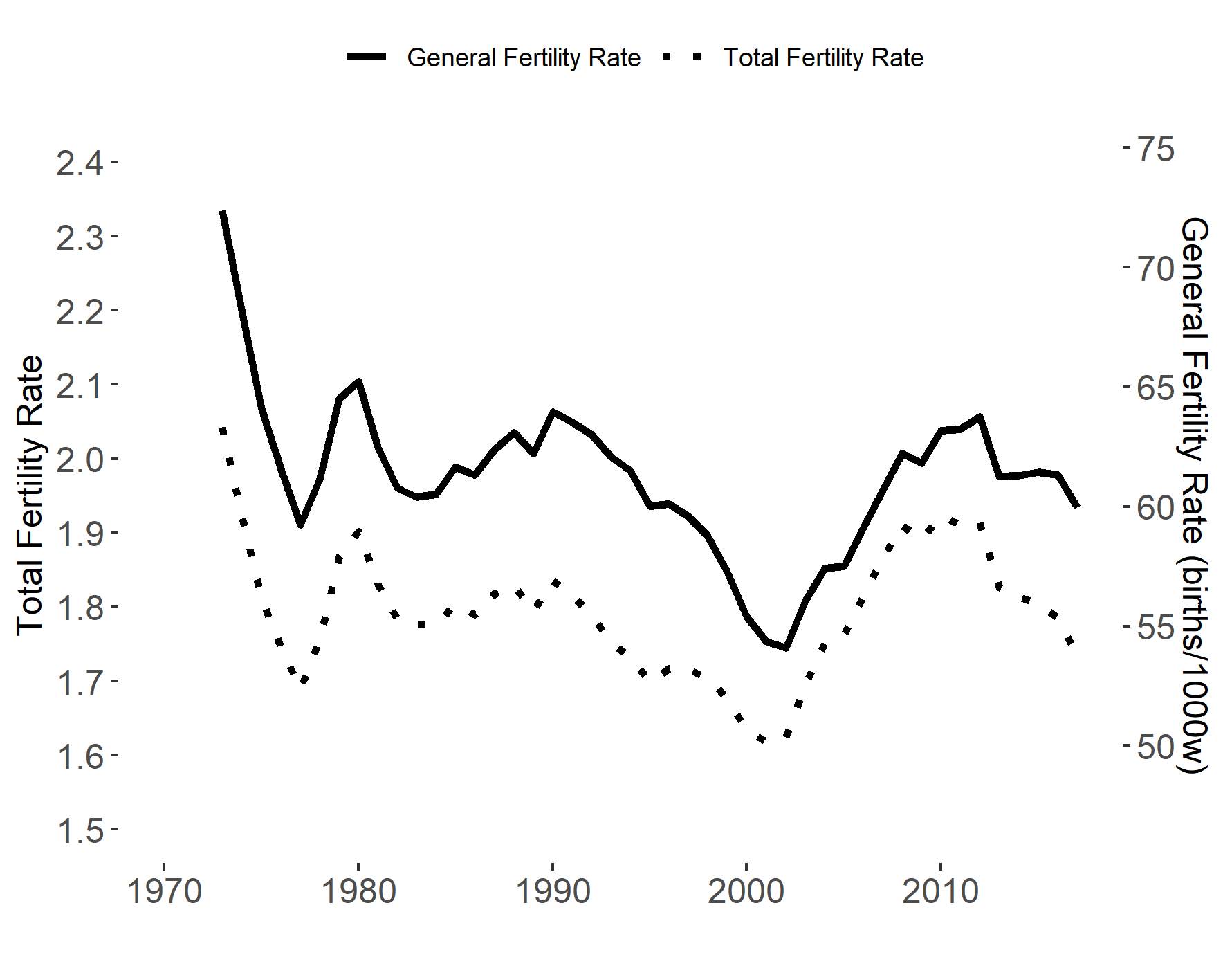
Figure 2.2: Fertility rates for the United Kingdom. Data source: Eurostat. Note: Only births of women aged 15-45 are included.
2.3.3 Relating the fertility measures to each other
Why do we have different fertility measures and what do they say? When thinking about fertility in layman’s terms, we typically think about the number of children a woman will give birth to in her life. It is an easily understandable hypothetical measure of fertility, which is captured by the Total Fertility Rate. It is hypothetical because we sum the age-specific fertility measures across ages at a given point in time. Any woman in this sample will of course only be included in one of the age specific fertility rates and contribute to that value. We impute the total fertility rate by summing over a lot of different age groups, who will be at different ages at different points in time.
The General Fertility Rate on the other hand gives information about the number of new children relative to the number of women of childbearing ages. It is therefore an actual (and not a hypothetical) number. This is a refinement of the Crude Birth Rate by taking into account the share of women in the population. To sum up, we should use the Total Fertility Rate to describe the fertility (behavior) and General Fertility Rate and CBR to describe the “number of individuals” added to the society. How does the General Fertility Rate relate to the Total Fertility Rate?
- The number of women in each age group varies
- The fertility rate varies across age groups.
If one of these sources is constant, the Total Fertility Rate will be the same as the General Fertility rate.
What can we learn from the chart?
So why did we combine the two line charts in Figure 2.2? Firstly, the goal was to investigate the link between these two series. The graph is scaled in a way such that the Total Fertility Rate should perfectly overlay the General Fertility Rate if they are the same (that is the level on the right vertical axis is equal to 31 times the corresponding value on the left axis). This is clearly not the case, but we see that the gap narrowed in the early 2000s. This will be the case if the age groups with higher age specific fertility rates are larger.
If every age group has the same fertility rates across years, but the number of people in an age group with a relatively high age specific fertility rate is larger next year compared to this year, the General Fertility Rate will increase, but the Total Fertility Rate will be unchanged.
2.3.4 Decomposing the development in childbirths
In the year 2000 the number of childbirths in England and Wales was 604,441. 16 years later, in 2016, the number of childbirths was 91,830 higher, at 696,271. What caused this increase? We can mechanically decompose this change into the two underlying factors:
- The number of women in England and Wales of childbearing age.
- The General Fertility Rate.
It could be the case that the number of childbirths increased because there are more women of childbearing ages. The fertility behaviour of these women was actually unchanged (in other words, the General Fertility Rate was constant). It could also be the case that the number of women of childbearing age stayed constant, but that the General Fertility Rate increased. Or it could be a mixture of both.
We can use the following formula to decompose the change in childbirths. Let \(\Delta X\) be the change in childbirths. We can then write this change as:
\[\begin{align} \Delta X&=Y_1\frac{X_1}{Y_1}-Y_0\frac{X_0}{Y_0}\nonumber\\ \Rightarrow &=\overbrace{Y_0\left(\frac{X_1}{Y_1}-\frac{X_0}{Y_0}\right)}^{A}+\overbrace{\left(Y_1-Y_0\right)\frac{X_0}{Y_0}}^{B}+ \overbrace{\left(\frac{X_1}{Y_1}-\frac{X_0}{Y_0}\right)\left(Y_1-Y_0\right)}^{C} \end{align}\]
Where General Fertility Rate is the ratio \(X/Y\) and the number of women of childbearing age is \(Y\).
- \(A\) captures the change in childbirths that is due to the change in General Fertility Rate.
- \(B\) captures the change that is due to a change in the number of women.
- \(C\) captures a combined effect of these changes.
Let’s apply this decomposition to the UK.
| Year | Live births (\(X\)) | Women aged 15-44 (\(Y\)) | General Fertility Rate (\(X/Y\)) | |
|---|---|---|---|---|
| 2000 | 604,441 | 10,812,898 | 0.0559 | |
| 2016 | 696,271 | 11,176,100 | 0.0623 | |
| Change | 91,830 | 363,201 | 0.0064 |
Using these numbers in the formula above, we get:
- \(A\) Change in fertility times number of women in 2000: \(0.0064*10,812,898=69,203\).
- \(B\) Change in the number of women times fertility in 2000: \(363,201*0.0559=20,303\).
- \(C\) Combined effect: \(0.0064*363,201=2,324\).
- Total change: \(A+B+C= 91,830\)
The decomposition shows that the change in the number of live births is mainly due to an increasing General Fertility Rate, the change in the number of women of childbearing age has, however, also contributed positively to the increase.
This decomposition method is not only applicable to fertility trends, but can be used for all changes that can be expressed as a ratio.
2.4 Calculating life expectancy
Having considered the flow of childbirths let us now move to the other important natural flow: deaths. To understand and explain changes in the number of deaths from year to year we can use the same approach as for the fertility rates above and consider the following two aspects:
- What is the population stock in each age group.
- What is the mortality rate in each age group.
The overall mortality over a period will increase if the mortality rates increase or if an age group with a higher mortality rate increases. A country can have a higher mortality rate than another country although all age-specific mortality rates are identical, because the age composition of the country differs. This comparison is just like comparing the General Fertility Rate (Or crude birth rate) across two countries.
While the Total Fertility Rate is a measure of the expected number of children that a woman will give birth to during her life, the Period Life Expectancy is a measure of the years a person can expect to live. However, although the intuition is the same, the computation of the Period Life Expectancy is slightly more complicated and we will therefore cover it in more detail.
Life expectancy is often considered one of the most important measures of social progress and it is often used in the public debate. The term “Life expectancy” seems quite intuitive. It answers an important question: how long can we expect to live? But how is it calculated? Just like with the Total Fertility Rate we compute the age specific mortality rates and then sum these in a given year. The life expectancy is therefore the number of years one can expect to live if one experiences the age specific mortality rates from that given year. However, we can have several children, but we can only die once. We therefore don’t create a hypothetical person, but a hypothetical cohort to calculate life expectancy.
Note that there is an alternative measure of life expectancy called cohort life expectancy. In that measure we follow a cohort. The data requirements are considerably higher for this approach, as we need to follow cohorts for the full life. We will here just capture period life expectancy which is also the most widely used measure.
2.4.1 Life tables
To calculate life expectancy we start by creating life tables. Life tables provide a list of period life expectancy for given age groups. Given you are in a specific age group today and given the mortality rates of each age group, what is your expected life expectancy. Table 2.2 shows the ingredients of life tables, where \(n\) is the width of the age intervals. If we are looking at variables by age in 1 year intervals we would set n=1. \(x\) is the specific age group. So \(x,x+n\) could refer to age interval 5 to 6, if x=5 and n=1.
| Col | Notation | Content | Source |
|---|---|---|---|
| (1) | \(x,x+n\) | The age interval | Provided |
| (2) | \(m_x\) | The age-specific mortality rate. | \(\frac{\text{deaths } x,x+n}{\text{population } x,x+n }\) |
| (3) | \(_nq_n\) | Prob. dying within interval. | \(\frac{2\times m_x}{2+ m_x}\) |
| (4) | \(I_x\) | Alive at age \(x\) | \(I_0=100,000\) |
| \(I_{x+n}=I_x-_nd_x\) | |||
| (5) | \(_nd_x\) | Number of people who die within interval. | \(I_x \times _nq_x\) |
| (6) | \(L_x\) | Person-years of life in interval | \(\frac{I_{x}+I_{x+n}}{2}\) |
| (7) | \(T_x\) | Cumulative person-years of life | \(\sum_{end}^x{L_x}\) |
| (8) | \(e_x\) | Average years of life remaining at age \(x\) | \(T_x/I_x\) |
2.4.2 The simple approach
Before we turn to the ingredients of Table 2.2 it is useful first to consider a simplified version.
We consider the life expectancy of mice (mice unfortunately have shorter lives than humans and they are therefore better suited for an example). You have the following data. This year 50 percent of all mice between age 0 and 1 died. 60 percent off all mice aged between 1 and 2 died. And all mice between 2 and 3 died.
Let’s create a simplified life table based on these statistics. We ignore \(_nq_n\) to make it simpler and consider an initial cohort of 10 mice. The table below shows a life table based on this information.
- Initially we have 10 mice. That is why the I column is 10 in row \(0-1y\). We know that 50 percent of mice in this age group died this year, so \(m_x\) is 0.5. That implies that 5 out of the 10 mice will die in this period, that is why \(ndx\) is 5. Looking at the next row, I is now 5 because out of the initial 10 mice, 5 died in the first year. 60 percent of the 5 mice die between before they turn 2, so we know that 3 of them will die in this age interval. We continue like this to fill out the first four columns,
In column \(L\) we enter the life years lived in this interval. So for the age group \(0-1y\) we know that 5 of the mice will survive this year so they will live five years in total (each mouse will live 1 year). For the remaining five mice we assume that they will die evenly throughout the year, meaning that they on average will live 0.5 year. So in total these five mice will live 2.5years, bringing the total up to 7.5years. We do the same in the next two rows.
Finally, in column \(T\) we add up how many live years there are left at this point. Starting for age group \(2-3y\), there are two mice who both will die. We assume that they die on average in the middle of the year, so they both can expect to live 0.5 years. 0.5 years times two mice gives 1 year. We do the same in row \(1-2y\) but here we also add the years left after they turn 2, so in total 4.5 and so on.
Finally in the last column we divide the total life years left by the number of mice at the beginning of that period, to get the average life years left for one mouse. As a result, the life expectancy at birth is 1.2y.
| age | Ix | \(m_x\) | ndx | L | T | e |
|---|---|---|---|---|---|---|
| 0-1y | 10 | 0.5 | 5 | 7.5 | 12 | 1.2 |
| 1-2y | 5 | 0.6 | 3 | 3.5 | 4.5 | 0.9 |
| 2-3y | 2 | 1 | 2 | 1 | 1 | 0.5 |
What was the simplifying step?
- We ignored that not everyone is born on the same day.
- We ignored that the likelihood of dying is not the same every day. At birth you are much more likely to die within the first 48hours than in the remaining year.
Incorporating these two extensions is what makes the “real” life table more complex. However, the intuition is the same.
2.4.3 Data requirements
For each age group we require data on the number of people in that group and the number of people who died in that group. Once we have these two variables we can construct the other variables. We can get such data from statistical agencies like Eurostat or the Office for National Statistics.
2.4.4 Creating life tables
The first variable we construct is the age specific death rate, followed by the probability of dying within the age group interval. We then construct a synthetic population that has a size of 100,000 individuals at the beginning of the first period. In each period we calculate the number of people who survive this period and who die within this period. We can then use these estimates to calculate the number of life years lived in this period, and sum over these live years. At the end, we divide the number of life years left in any given period by the number of people getting to this period to obtain the estimated life expectancy.
| age | mx | nqx | ndx | Ix | Lx | Tx | ex |
|---|---|---|---|---|---|---|---|
| 0 | 0.004 | 0.004 | 385.000 | 100,000 | 99,808 | 8,081,572 | 80.816 |
| 1 | 0.000 | 0.000 | 25.376 | 99,615 | 99,602 | 7,981,765 | 80.126 |
| 2 | 0.000 | 0.000 | 14.013 | 99,589 | 99,582 | 7,882,163 | 79.147 |
| 3 | 0.000 | 0.000 | 11.453 | 99,574 | 99,568 | 7,782,581 | 78.159 |
| … | … | … | … | … | … | … | … |
| 98 | 0.346 | 0.295 | 980.052 | 3326 | 2836 | 3128 | 0.941 |
| 99 | 0.386 | 0.324 | 758.769 | 2345 | 293 | 293 | 0.125 |
Table 2.2 shows a subset of a life table for the United Kingdom using data from Eurostat and the recipe outlined in Table 2.4. The table shows that the life expectancy at birth is 81 years. Conditional surviving to age 99, the life expectancy is 0.125 years. However,the life expectancy at higher ages is highly influenced by the assumption that all individuals die at a given age. In this case it is by age 100 years. In Figure 2.3 we plot the variable \(e_x\) against \(x\) from the life table and life.
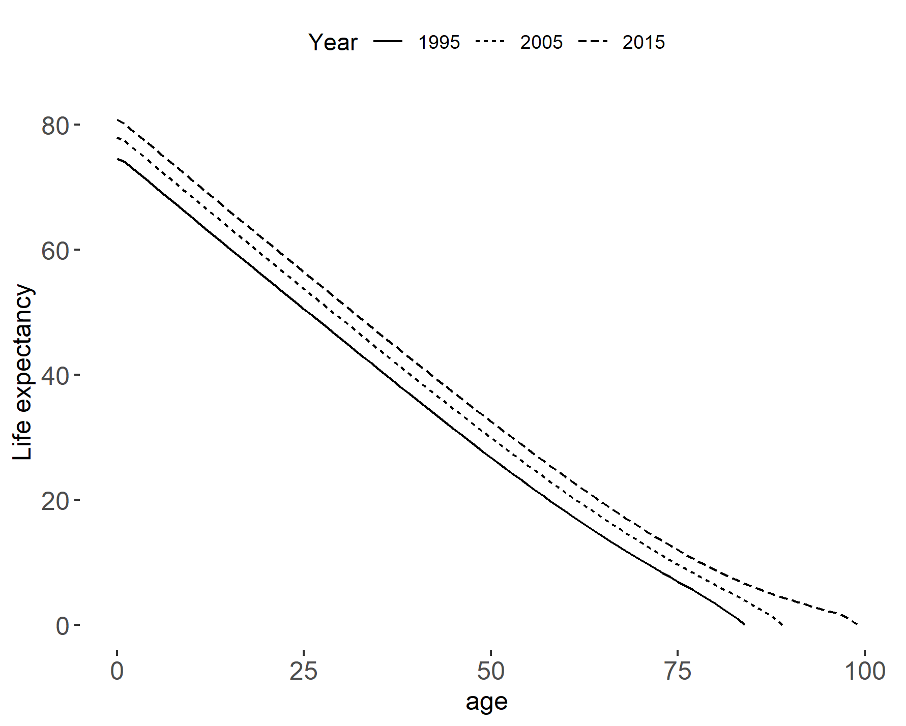
Figure 2.3: Life expectancy by age in years (left) and survival probabilities (right). Data source: Eurostat.