4 Economic Activity

4.1 What this chapter is about

This chapter is about economic activity. Along with the unemployment rate, economic activity is one of the most used economic concepts in policy discussions. What is it? What does it capture? And importantly, what does it not capture?

Economic activity is measured in the System of National Accounts (SNA) and conceptualized by the Gross Domestic Product, (GDP). We will not cover the SNA in detail.² The System of National Accounts is basically big bookkeeping of economic transactions in a region over a given period of time. The SNA includes a set of rules and instructions that have been agreed upon internationally to ensure that measures of economic activity are comparable across countries. In this chapter we will go through some of the key aggregates of the SNA, for example Gross Domestic Product, a measure of economic activity. An aggregate is a measure that aggregates several underlying variables. This chapter is mainly about the GDP, but we will also briefly touch upon other aggregates of the SNA as well as what the GDP is used for.

4.1.1 Intended learning outcomes

After reading this chapter you should be able to:

• Explain what the gross domestic product (GDP) is and calculate it.
• Explain the three ways to measure GDP
  1. The Income Approach
  2. The Expenditure Approach
  3. The Output approach.
• Explain what the gross national income (GNI) is and calculate it.
• Calculate GDP per person and productivity.
• Visualize data on economic activity.

4.2 A super brief history of GDP

Most texts about the history of GDP start around the Great Depression in the 1930ies United States. The US Congress realised that the economy was not doing as well as it could, but had a hard time quantifying how bad the situation actually was. To the “rescue” came the economist Simon Kuznets who provided a report on the “National Income, 1929-1935” for the Congress (see 4.1), where he presented the idea of capturing the entire production, income and expenditure of the economy. And so the modern concept of GDP was born. However, measures of economic activity have existed for many years.

Figure 4.1: Kuznets’ report for the U.S. Congress, 1934. Source: Fraser St. Louis FED.

The idea of quantifying the size of the economy probably goes back to at least the 17th century. The exact definition of GDP has since then been redefined and adjusted. It is actually continuously adjusted. More on that later. Giving Simon Kuznets a lot of credit for the GDP is not completely wrong. He refined the concept a lot and his report made it prominent. However, it wasn’t until much later that it became the “statistic to rule them all”.

The GDP as a concept is criticized a lot. The most prominent criticism is probably the “Report by the Commission on the Measurement of Economic Performance and Social Progress” published in Autumn 2009 by the economists Joseph Stiglitz, Amartya Sen and Jean-Poul Fitoussi. What is the key criticism of GDP? The main problem with the GDP is not so much the GDP itself, but more the use and policy focus on GDP as a measure of well-being or welfare. Simon Kuznets was actually already aware of some of these issues and the potential misuse of GDP. Figure 4.1 shows a small section of the 273 page long report by Kuznets.

Figure 4.2 shows extracts of pages 5-7 in Kuznets original report.³ Kuznets made several points that are at the heart of the discussion today, for example that “With quantitative measurements especially, the definiteness of the result suggests, often misleadingly, a precision and simplicity in the outlines of the object measured.” and “Economic welfare cannot be adequately measured unless the personal distribution of income is known. And no income measurement undertakes to estimate the reverse side of income, that is, the intensity and unpleasantness of effort going into the earning of income.”

Figure 4.2: Page 5-7 in ‘National Income, 1929–1932’. 73rd US Congress, 2d session, Senate document no. 124, 1934. Source: Fraser St. Louis FED.

So why should we care about GDP if it is no good? Because the GDP is a reasonably good of market economic activity. We will return to the criticism of GDP in later chapters, but here we will discuss what it actually captures. When we know what the GDP measures, we can say more about what it doesn’t measure and how we should and should not use it.

4.3 The Economy of Microcountry

“…ordinary business of life” in Microcountry

Let me introduce a very small country. It is not my home country, Denmark, but a country that is even smaller: Microcountry. Microcountry is just next to Neighbourcountry. Microcountry is so small that I can explain all economic activity in this country to you in a few paragraphs.

In Microcountry we have one farm that produces flour. The farm sells the flour to a bakery for 10 £. To produce the flour, the farm has workers, and these workers earn a wage of 8 £. Finally, the farm pays a tax to the government of 2 £.

The bakery produces bread based on labor inputs in terms of workers and the flour bought from the farm. The workers at the bakery receive 14 £ in wages, and the government receives 2 £ in taxes from the bakery. The bakery sells bread for 18 £ to the households in Microcountry. The households of Neighbourcountry buy bread from the bakery in Microcountry for 9 £, and the bakery in Microcountry is actually owned by residents of Neighbourcountry.

The households in Microcountry work for the bakery, the farm and for the government. They pay 1 £ in taxes to the government, and buy bread for 18 £ at the bakery. The households also import cheese from Neighbourcountry for a value of in total 8 £. The Government provides health service and a school for the residents of Microcountry and spend 5 £ in wages to teachers and health providers to be able to supply this service.

Quantifying economic activity in Microcountry

So we know that the people in Microcountry go to work at a farm, in a bakery, in a school or in health services. We know that they buy bread and cheese. These activities are just examples of “…ordinary business of life” (from Alfred Marshal’s quote “[…] economics is a study of mankind in the ordinary business of life” in The Principles of Economics). How can we quantify these economic activities?

What is economic activity? Just think of when you are economically active:

1. When you go shopping and spend money.
2. When you work and receive a wage, and when you earn profits.
3. When you create a product and sell it to someone.

These three examples of how we as individuals are economically active actually capture the three ways we measure the Gross Domestic Product (GDP). The expenditure approach, the income approach and the output approach. Let us now discuss these approaches in detail. The GDP captures how much is spent, how much is produced or how much is earned within a period. It is therefore a flow variable.

You know basically know how to measure GDP. Just consider the sum of all expenditures in Microcountry. Or the sum of all income generated. Or the sum of all output created. All these approaches give the same value. Try it on the Microcountry above. You will probably realise that it is slightly more complicated. We will therefore cover this in more detail below.

Before we turn to the description of the measurement approaches, here is a short video of what the GDP is, created by the UK Treasury.

Figure 4.3: What is GDP?. Source: HM Treasury.

4.4 The 3 ways to measure GDP

The Expenditure Approach

The expenditure approach (called the spending approach in The Core) measures the GDP in terms of expenditures by households and the Government, as well as investments and net exports of goods and services (i.e. exports minus imports). All these expenditures are summarised by the following equation: \[\begin{align} \text{GDP}^{\text{E}} \text{=Y=C+G+I+X-M} \end{align}\] where:

• Y is the Gross Domestic Product (GDP).
• C is the final consumption of goods and services by households. It includes goods like food, cars, and clothing, as well as services such as hotel stays.
• G is the final consumption expenditure of goods and services by the government.
• I are the investments (also called gross capital formation) in fixed assets such as machinery, buildings etc.
• X is goods and services produced domestically but consumed abroad (Exports)
• M is goods and services produced abroad and consumed domestically (Imports).

Let us return to Microcountry and use the expenditure approach to calculate the economic activity of Microcountry.

• \(C\) household consumption:
  • The households buy bread at the bakery for 18£ and import goods from Neighbourcountry for 8£, \(C=8£+18£=26£\).
• \(G\) Government consumption:
  • The government spends 5£ on health services, \(G=5£\).
• \(I\) Investments:
  • There are no investments in this economy, \(I=0£\).
• \(X\) Exports:
  • The bakery exports bread to Neighbourcountry for 9£, \(X=9£\).
• \(M\) Imports:
  • Microcountry imports goods for the value of 8£ from Neigbourcountry, \(M=8£\).

The GDP of Microcountry is therefore \(Y=26£+5£+9£-8£=32£\).

Let’s now move to a real economy, the United Kingdom. In the following Table we show the expenditure approach to calculate GDP for the United Kingdom. Private consumption, that is our \(C\), constitutes for about two-thirds of the GDP. Government consumption, \(G\), constitutes for 18%, Investments, \(I\), constitute for 17%, and Net exports are only slightly negative (as Imports are larger than Exports).

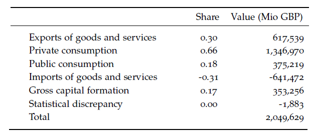
(#fig:gdpexp_)Gross Domestic Product of the United Kingdom using the expenditure approach, in 2017.Data source: OECD. All values are in 2017 prices.

The income approach

A second approach to measuring GDP is the income approach. The income approach measures the GDP in terms of the generated income in the economy. The income generated in an economy consists of all compensation to workers (wages, pension contributions etc.), operating surplus (profits and rents) and sales taxes minus subsidies.⁴

\[\begin{align} \text{GDP}^{\text{I}} \text{=W+P+NT} \end{align}\] where

• W is worker compensation.
• P is operating surplus.
• NT is sales taxes minus subsidies.

Let us return to Microcountry and use the income approach to calculate the economic activity of Microcountry.

• \(W\),worker compensation:

  • The farm workers receive a wage compensation of 8£, the bakery workers receive a wage compensation of 14£ and the health service workers receive a compensation of 5£. The total wage compensation is therefore \(W=8£+14£+5£=27\).

• \(P\), operating surplus:

  • The farm has zero profits, but the bakery has a profit of 1£, \(P=1£\).

• \(NT\), taxes minus subsidies:

  • The farm pay 2£ in taxes and the bakery pays 2£. There are no subsidies. The taxes minus subsidies are therefore, \(NT=2£+2£=4£\).

The GDP of Microcountry is therefore \(Y=27£+4£+1£=32£\).

Let’s now move back to the real economy of the United Kingdom. In the following Table we show the income approach to measure GDP for the United Kingdom. Compensation of employees, that is our \(W\), constitutes for about half of the GDP. Profits, \(P\), constitute for 38%, and the remaining 12% are net taxes.

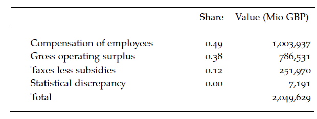
(#fig:gdpexp_2)Gross Domestic Product of the United Kingdom using the income approach, in 2017.Data source: OECD. All values are in 2017 prices.

The production approach

The third and last approach to measuring GDP is the production approach (also known as the output approach). So far we have considered how much we’ve spent (the expenditure approach), how much income was generated (the income approach) and now we finally look at how much we produced. The production approach measures the GDP in terms of production or value added. The value added is the value of the output minus the costs of the intermediate goods. If a bakery buys flour for 15 £ and sells bread for 50 £, the value added by the bakery is 50-15=35 £. Intermediate goods are all goods used in the production process, such as raw materials, fuel, rental costs, cleaning and marketing costs.

We typically distinguish between two types of outputs, market and non-market outputs. The market outputs are goods and services sold on the market, such as the bread sold by the bakery. In that case the value added is straightforward to calculate, as it is the sales price minus the price of the intermediate goods. However, not all goods are necessarily sold, so we also include the change in inventories. For non-market output, such as health and defence, the output is the production costs, i.e. the cost of labor and intermediate goods (and depreciation in fixed assets). Finally, there is a distinction between value added in basic prices and value added in market prices. To obtain the latter we have to add sales tax and subtract subsidies.

\[\begin{align} \text{GDP}^{\text{P}} \text{=GVA+NT} \end{align}\] where

• GVA is gross value added.
• NT is taxes minus subsidies.

Let us return to Microcountry and use the expenditure approach to calculate the economic activity of Microcountry.

• \(GVA\), gross value added

  • The farm sells flour for 10£ and pays 2£ in taxes. The gross value added of the bakery is therefore 8£. The bakery sells bread for 27£, pays a sales tax of 2£ and pays 10£ for the flour from the bakery. The gross value added of the bakery is therefore 15£. Finally, the public sector provides a health service. The value of public sector provision is typically estimated by means of the costs, which in this case is 5£. The total gross value added in Microcountry is therefore $GVA=8£+15£+5£=28£.

  • The farm pays 2£ in taxes and the bakery pays 2£. There are no subsidies. The sales taxes minus subsidies are therefore, \(NT=2£+2£=4£\).

The GDP of Microcountry is therefore \(Y=28\)+4£=32£.

Finally, let’s now move back to the real economy of the United Kingdom. In the Table below we show the production approach to measure GDP for the United Kingdom. In this example we show Gross Value Added separately by sector. This is one of the advantages of having several measures of GDP: We can decompose the GDP into different dimensions. In this example we observe that Public services and distributive trades are some of the largest elements of the UK GDP.

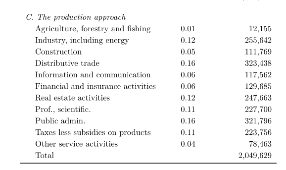
(#fig:gdpexp_3)Gross Domestic Product of the United Kingdom using the production approach, in 2017.Data source: OECD. All values are in 2017 prices.

4.4.1 What is included in the GDP measure?

Measuring GDP also requires us to understand which activities we should include, and which we should not include. Based on the general principles described in the ESA 2010, the Office for National Statistics decides on a production boundary, which contains all economic activities that should be included in the GDP measurements. An activity is included in the boundaries if:

• The activity produces a meaningful output.
• The product or activity has a meaningful market value, or the market value can be imputed.
• The inclusion of the activity increases the meaningfulness of cross-country comparisons.

Several activities are less clear-cut than you might think, for example activities where “production is forbidden by law; as long as all units involved in the transaction enter into it voluntarily” are included. Breeding of fish in fish farms is included, but breeding of fish in open seas is not included.

4.4.2 GDP - Why 3 approaches?

Note how all three approaches show the same results in form of the same GDP. For simplicity, one might therefore argue that we should just stick to one approach and ignore the two other approaches. However, each approach has its own advantage. First,the expenditure approach is very useful if you want to assess whether changes in GDP are driven by for example domestic consumption or exports. Moreover, we can decompose all approaches in more detail. We could for example identify which sector is contributing most to the value added using the production approach. While the three approaches in theory should lead to exactly the same number, we often observe small discrepancies in practice. These discrepancies are called “statistical discrepancy”.

Measuring GDP - an overview

1. The expenditure approach

• The expenditure approach (called the spending approach in ⁵) measures the GDP in terms of expenditures by households and the Government, as well as investments and net exports of goods and services (i.e. exports minus imports).

\[\begin{align} Y=C+G+I+X-M=C+G+I+NX \end{align}\]

• Y is the Gross Domestic Product (GDP).
• C is the final consumption of goods and services by households. It includes goods like food, cars, and clothing, as well as services such as hotel stays.
• G is the final consumption expenditure of goods and services by the government.
• I are investments (also called gross capital formation) in fixed assets such as machinery, buildings etc.
• X is goods and services produced domestically but consumed abroad (Exports)
• M is goods and services produced abroad and consumed domestically (Imports).

2. The income approach

• The income approach measures the GDP in terms of the generated income in the economy.

\[\begin{align} Y=W+P+NT \end{align}\]

• W is worker compensation.
• P is operating surplus.
• NT is sales taxes minus subsidies.

3. The production approach (also known as the output approach)

• The production approach measures the GDP in terms of production or gross value added.

\[\begin{align} Y=GVA+NT \end{align}\]

• GVA is gross value added.
• NT is sales taxes minus subsidies.

4.5 Gross National Income (GNI)

Gross national income (GNI) is the income received by residents of the domestic economy. The GNI is thus defined as the GDP plus the net property income from abroad. Where property income consists of interests, rent on land and income from corporations. The GDP and GNI can be very different. If for example most firms in the economy have foreign owners, the profits of these firms will be subtracted from the GDP, and the GNI will thus be considerably lower.

Let’s look at Microcountry. We found a GDP of 32£ independent of how we measured GDP. However, because the bakery is owned by residents in Neighborcountry, the profits go abroad, and the Gross National Income is: $GNI=32£-1£=31£.

4.6 What we use GDP for

Now what do we need these measures for? The GDP is an important aspect in many policymakers evaluation of the condition of the economy. For example, during the Great Depression in the late 1920ies and early 1930ies the economy looked quite bad, but how bad was actually hard to describe. The United States congress therefore asked the economist Simon Kuznetz to quantify US economic activity. Kuznetz’s estimates gave the first insights into the magnitude of the Great Depression by showing the change in economic activity during the great depression. Let us just consider a few uses of GDP.

1 Growth rates

As it was the case during the Great Depression, we are in general typically more interested in changes than in levels of GDP. It is maybe the most popular statistic of policy makers: the growth rates. Getting from the level of GDP to the growth rates is straightforward, given that the levels are measured in real terms, that is at a constant price level (we will return to the issue of real and nominal terms in later chapters). We can use the following formula to calculate the growth rate in percent:

\[\begin{align} \text{growth rate in percent}=100\times \left(\frac{GDP_t}{GDP_{t-1}}-1\right) \end{align}\]

In this expression the letter \(t\) refers to the time period. This could be a year, a quarter or a month. Figure 4.4 shows the GDP of the UK using a fixed price level and the annual growth rates. The yearly growth rates roughly correspond to the first derivative of the level, as they show the changes. Therefore, we are actually able to identify the large dip in 2009 even at the levels shown in the graphs above. However, identifying whether growth rates are 2 or 3 percent is difficult based on the levels, and bar charts of growth rates are therefore a very common way to visualize the economic conditions.

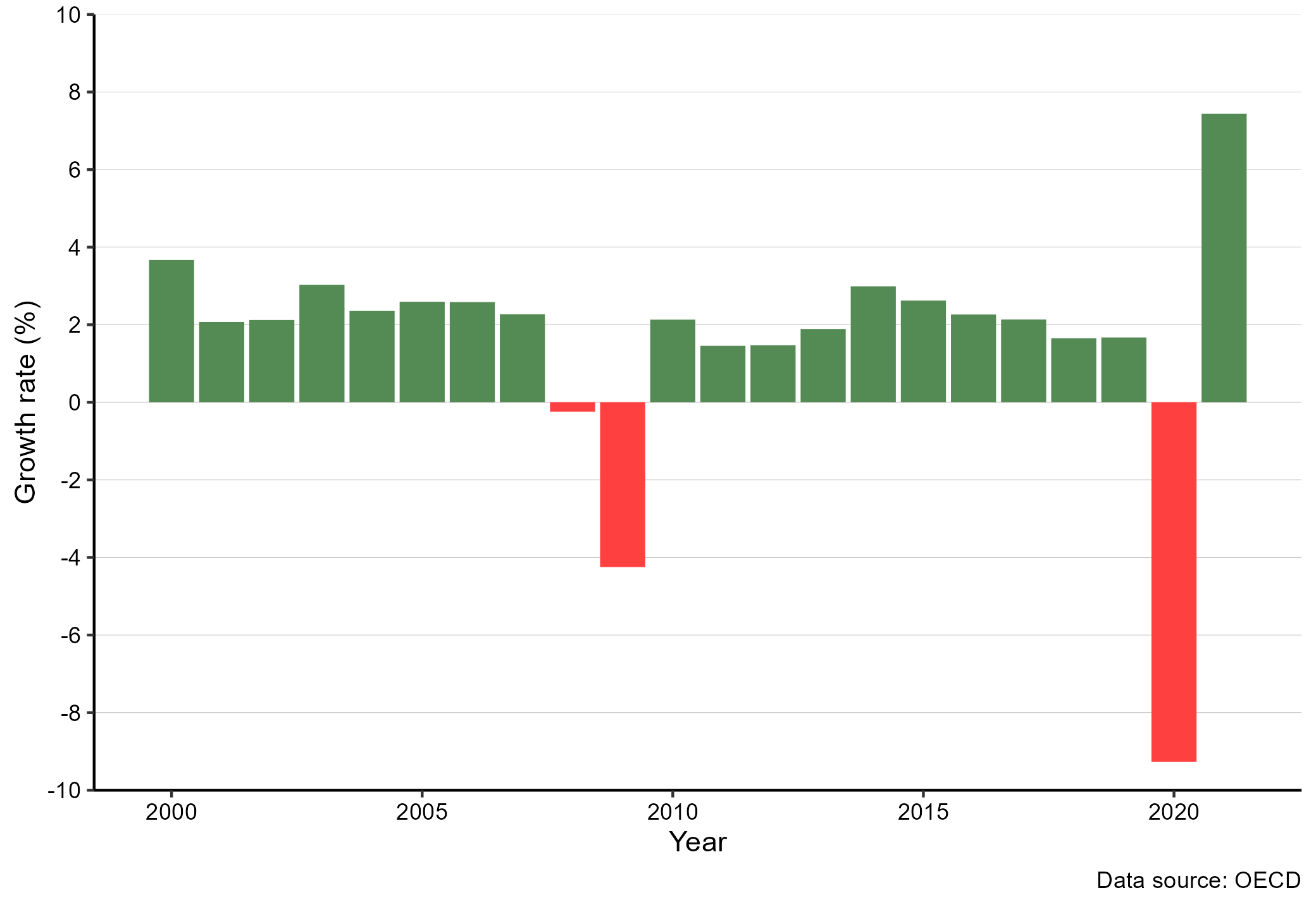
Figure 4.4: Annual GDP growth rates for the UK, 2000-2018. Using a bar chart. Source: OECD. The GDP level is measured in terms of the 2017 price level.

2 Decompose growth

We can use each of the GDP measurement approaches above to decompose the overall GDP growth. Using the expenditure approach, we could calculate the overall GDP growth as follows:

\[\begin{align} growth\text{ }rate=&I's growth\text{ }rate\times I's\text{ }initial\text{ }share\text{ }of\text{ }GDP\\ &+G's growth\text{ }rate\times G's\text{ }initial\text{ }share\text{ }of\text{ }GDP\\ &+C's growth\text{ }rate\times C's\text{ }initial\text{ }share\text{ }of\text{ }GDP\\ &+NX's growth\text{ }rate\times NX's\text{ }initial\text{ }share\text{ }of\text{ }GDP \end{align}\] In words, the overall GDP growth is simply a weighted average of each component’s growth rate. The weights are the share of overall GDP in the initial period.

Why is this useful? Say we wanted to know how household consumption \(C\) contributed to GDP growth. \(C's\) contribution is given by: \(growth\text{ }in\text{ }C\times C's\text{ }share\text{ }of\text{ }GDP\), which we can relate to the overall growth:

\[\begin{align} C's\text{ }contribution\text{ }to\text{ }growth=\frac{growth\text{ }in\text{ }C\times C's\text{ }share\text{ }of\text{ }GDP}{overall\text{ }GDP\text{ }growth} \end{align}\]

3 Business cycles

Once we know the changes in economic activity, we can start characterizing periods by terms such as business cycles, booms, overheating and recessions. The actual definitions of these concepts are considerably less clear. The US National Bureau of Economic Research has a “Business Cycle Dating Committee” that specifies the chronology of the US business cycles. The committee does not have a fixed definition of recessions. Instead they combine real GDP, with data on the labour market and data on income. However, their definitions of recessions often coincide with a definition based on two consecutive quarters of decline in real GDP.

How exactly expansions and recessions are identified varies from country to country, but in the European Union we typically define a recession as two successive quarters of negative economic growth. A business cycle is typically defined as the period from a boom to recession and back to boom, in other words, from peak to peak. Figure 4.4 shows annual levels, and we clearly see a drop in real output in 2008 and 2009. In terms of quarters, the growth rate was negative from the second quarter of 2008 to the second quarter of 2009.

GDP and business cycles

• An economic recession is the period from peak economic activity to the lowest level of economic activity.
• An economic expansion is the period from the lowest level of economic activity to the highest level of economic activity.
• The economic cycle of recessions and expansions is called business cycles.
• There is no general stringent definition of a recession, but two consecutive quarters of decline in real GDP is often seen as a sign of a recession.

4 GDP per capita

While GDP growth rates are used across time, we are sometimes also interested in comparing across regions or countries. First, we could be interested in identifying regional recessions and expansions. Second, we could be interested in comparing the level of economic activity per capita. To achieve the latter, we divide data on the total GDP for each region or country and divide by the number of residents in the region or country. Figure 4.5 shows the economic activity per person in 2015. We have adjusted the price levels to be comparable across time and space. In this chart the values correspond to the price level of 2017 and we have adjusted all national values to the US price level and show the values in US dollars. To be clear, we do not simply use the exchange rate to translate the national currencies, but we also take differences in price levels across countries into account. Luxembourg has, by far, the highest level of economic activity per person, followed by Ireland and Switzerland. Of the OECD data with available data, Chile has the lowest GDP per person.

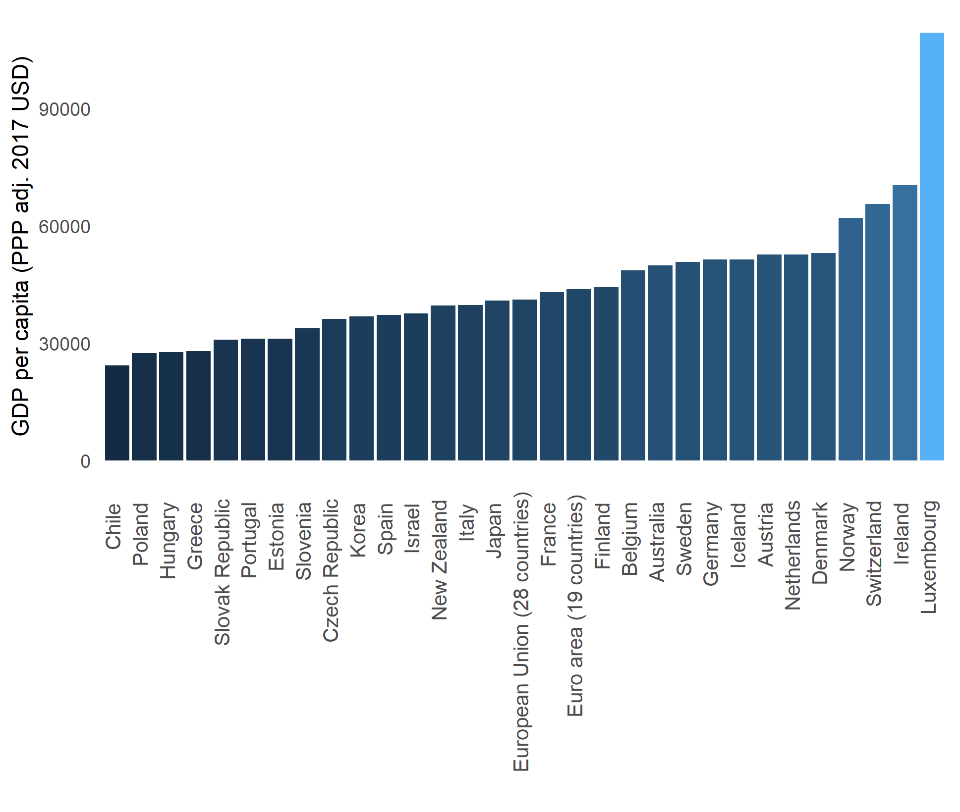
Figure 4.5: GDP per capita for selected countries in 2015, measured in 2017 USD - PPP adjusted. Source: OECD.

Figure 4.6 shows the relative change in real economic activity per person from 2000 to 2015. Most countries increased the output per person, but not all.

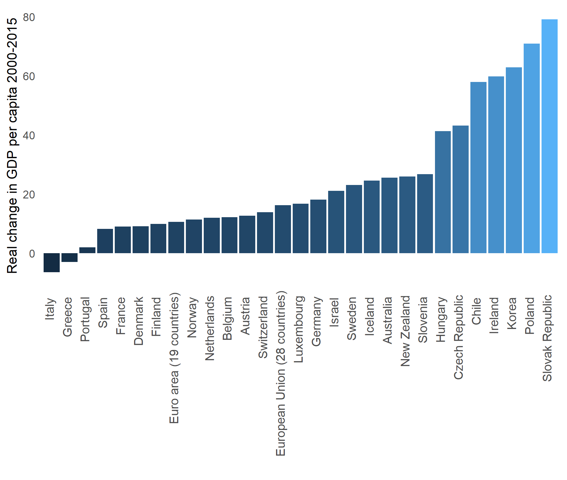
Figure 4.6: Real change in GDP per capita for selected countries 2000-2015, real values measured in 2017 USD - PPP adjusted. Source: OECD.

Productivity

Productivity is a measure of how much we can produce relative to the resources used in the production. A higher productivity means that we produce more given resources (or produce the same with fewer resources).

A very common approach is to measure the Gross Value Added per worker or per hour worked. A higher value then suggests that we can produce a greater value added with fewer labor inputs. However, we could also consider other inputs such as capital. However, the most simple approach is probably GDP per worker. This is closely related to GDP capita, which we discussed above, but in this approach we only consider the individuals who are in the labor market. Using this approach we can provide a crude but straightforward indicator for the labor productivity of a country. Changes in productivity are often the first step in understanding changes in economic activity.

The balance of trade

The balance of trade is the difference between exports and imports, also called net exports and denoted \(NX\):

\[\begin{align} NX=X-M \end{align}\]

• NX is the balance of trade or net exports.
• X is goods and services produced domestically but consumed abroad (Exports)
• M is goods and services produced abroad and consumed domestically (Imports).

If the balance of trade is positive it means that a country has a trade surplus, because it exports more than it imports. If a country imports more than it exports, in other words, when the trade balance is negative, the country has a trade deficit.

Balance of payments

The balance of payments (BoP) captures the overall transactions between a country and the rest of the world. The “balance” means that the sum of the current account, financial account and capital account has to be zero.

• The current account consists of the balance of trade (as defined above) and the income balance (income earned abroad from domestic residents minus income earned by foreign residents).
• The capital account captures international capital transfers.
• The balancing item captures statistical inaccuracies.

\[\begin{align} \text{current account}+\text{capital account}+\text{balancing item}=0 \end{align}\]

Let’s consider an example: If we go to Germany on holiday and spend 10£ in restaurants and hotels using our English credit card, we are causing a 10£ debit on the trade balance. Let’s say that we also export some English Breakfast tea for the value of 100£ to Germany. This is noted as a 100£ credit on the trade balance. The balance of trade is then \(100£-10£=+90£\). We don’t earn anything abroad and no foreigner earned something in England. The current account would then be \(+90£\).

Now let us look at the capital account. The 10£ spent abroad using our English credit card will be recorded in our capital account as an investment. If we also buy some German stocks for say 15£, then these stocks will appear in debit as “portfolio investment”. However, because we use our English credit card to buy these stocks, the 15£ will also appear on our capital account as a credit (just like the hotel and restaurant shopping). Finally, the trade credit payment from the German tea buyer is recorded in the financial accounts as a debit. The net capital account is then \(25£-115£=-90£\). As expected, the sum of the current account plus the capital account is zero. This occurs by definition through the double entry accounting framework (each entry is entered both as a debit or a credit).

It is common to separate out “financial account” from the capital account and use this extended definition: \[\begin{align} \text{current account}+\text{capital account}+\text{financial account}+\text{balancing item}=0 \end{align}\]

4.7 Further readings

• GDP and Me by the ONS
• What is GDP by the ONS
• What is GDP by the Bank of England