5 Designing Tables in Microsoft Excel

5.1 Basic cell formatting

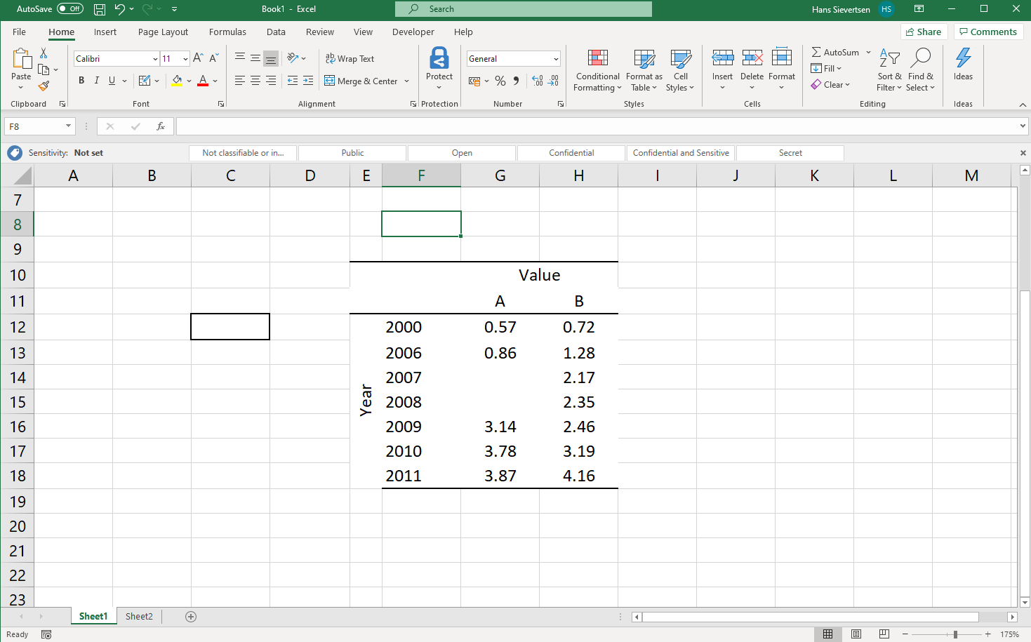
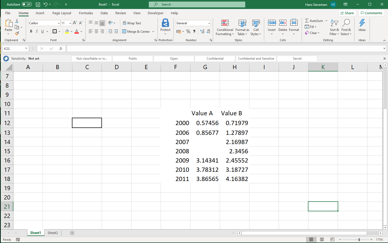
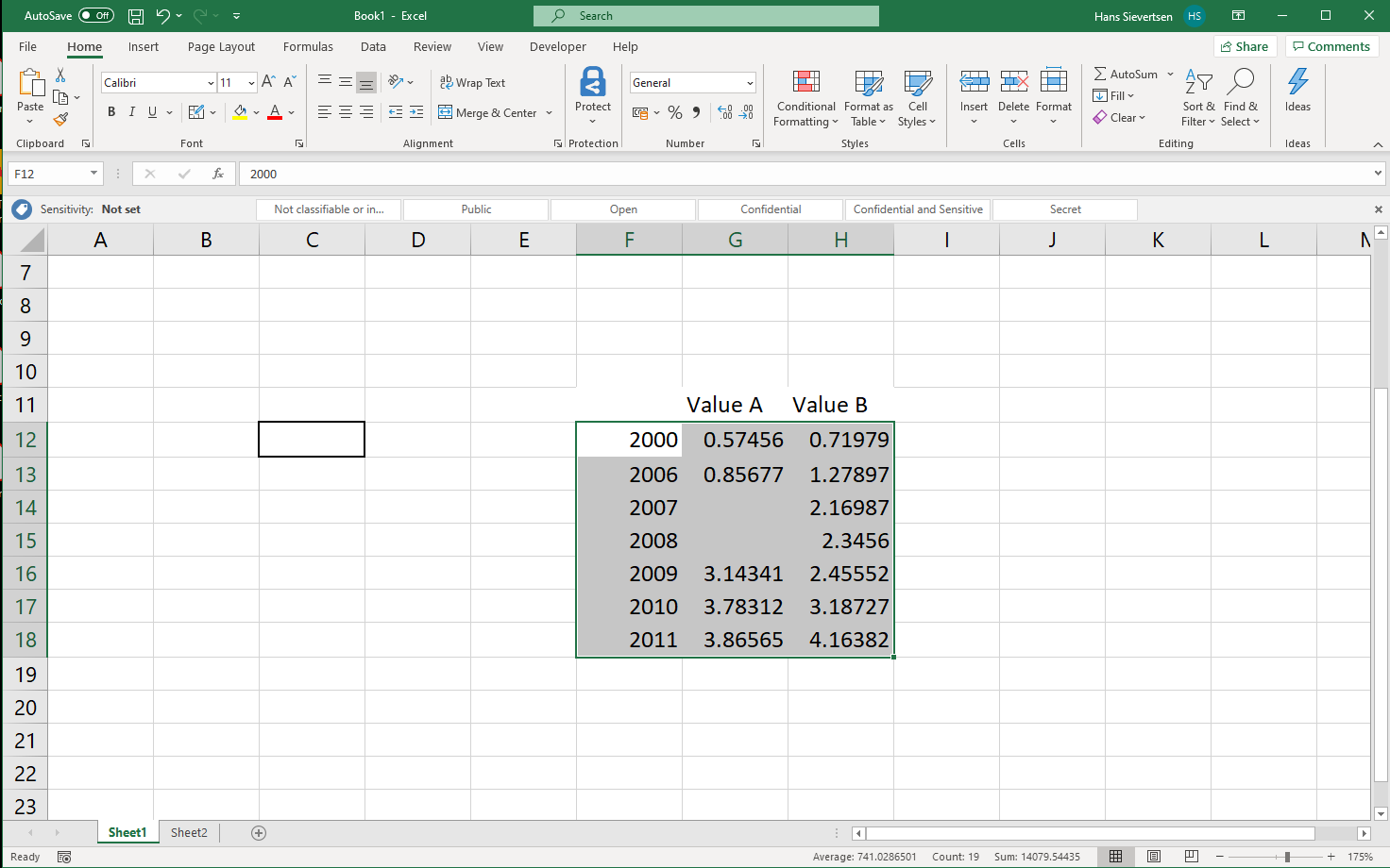
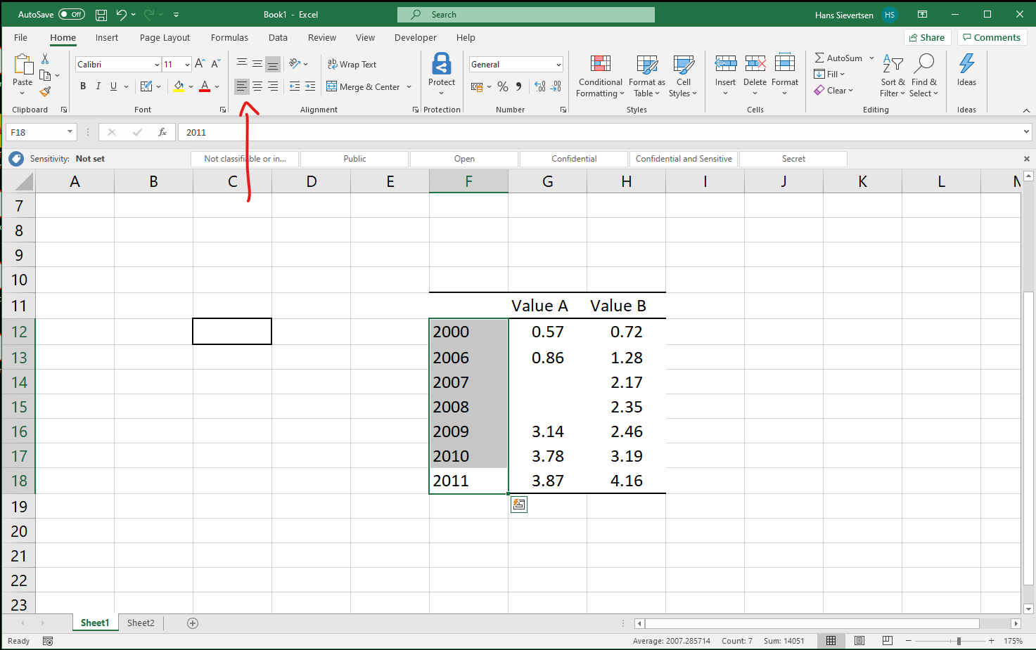
Consider the table below. It shows the values for two series, “Value A” and “Value B” over years. Let’s for now assume that we are happy with the structure of the table and we just want to improve the design. This includes

1. The colour and thickness of lines.

2. The alignment of values and labels.

Modifying Borders

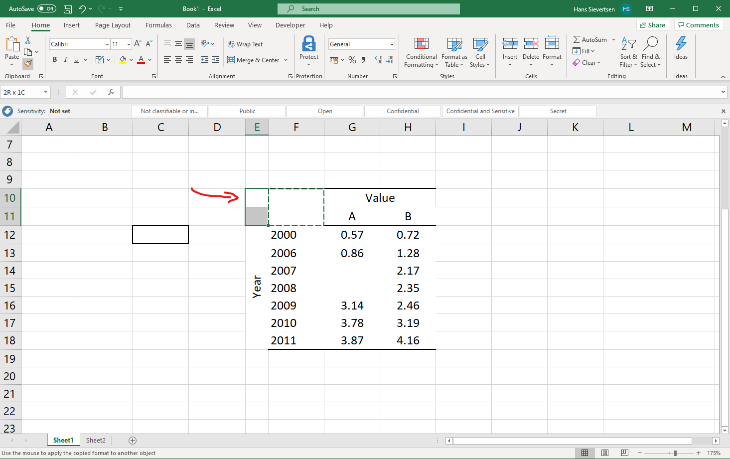
We can add solid black orders to a selected cell by clicking on the “Borders” icon (see arrow below) in the “Home” tab ribbon.

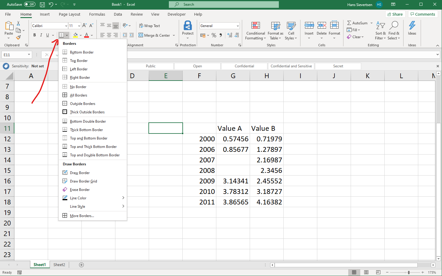
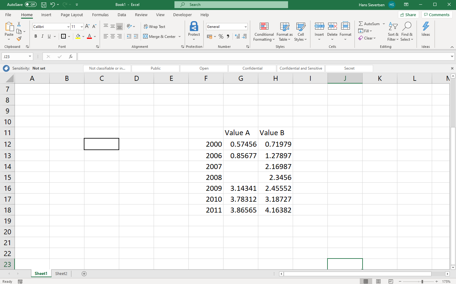
Below is an example where cell C12 is given a solid black line as a border on all sides.

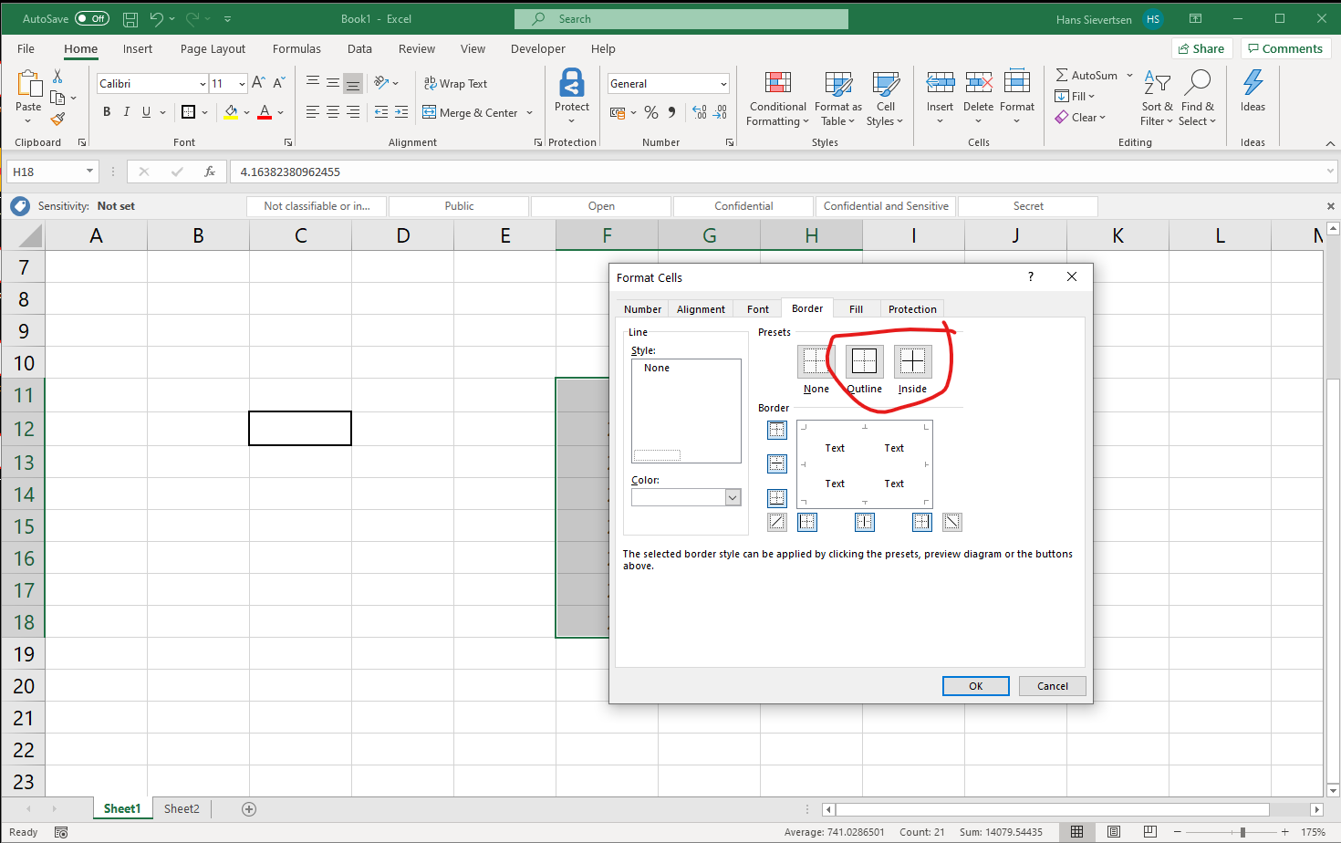
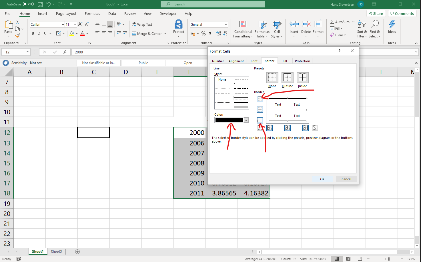
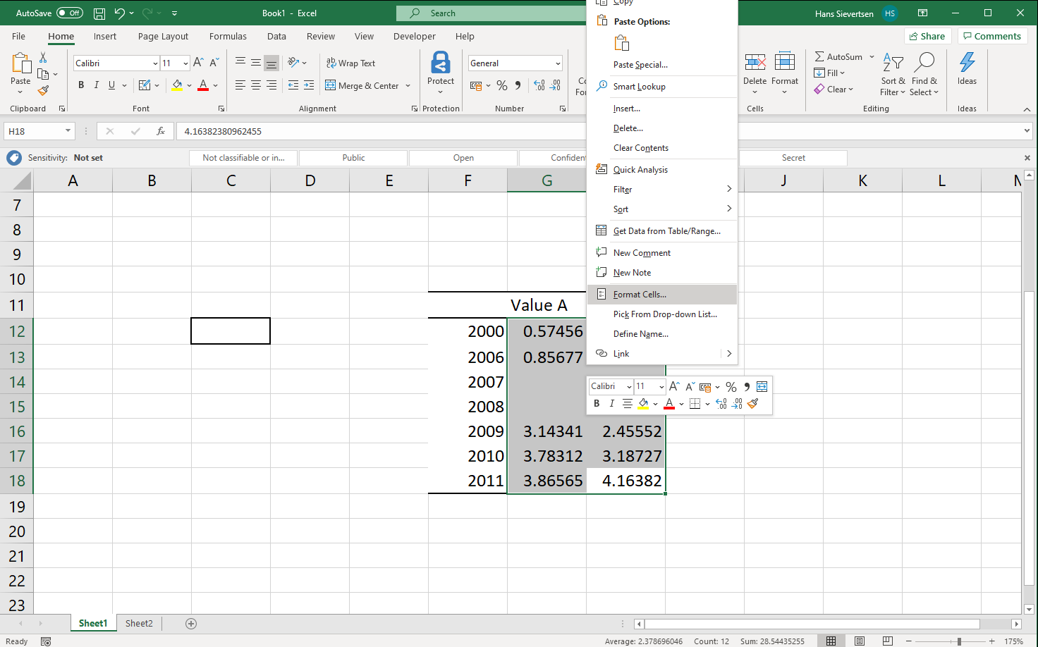
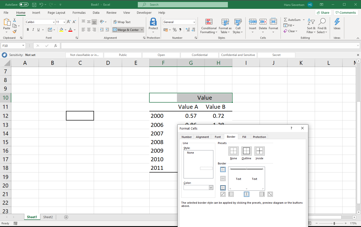
An alternative approach to modifying borders is to select a range of cells, right-click on the selected area, and select “Format Cells” as shown below.

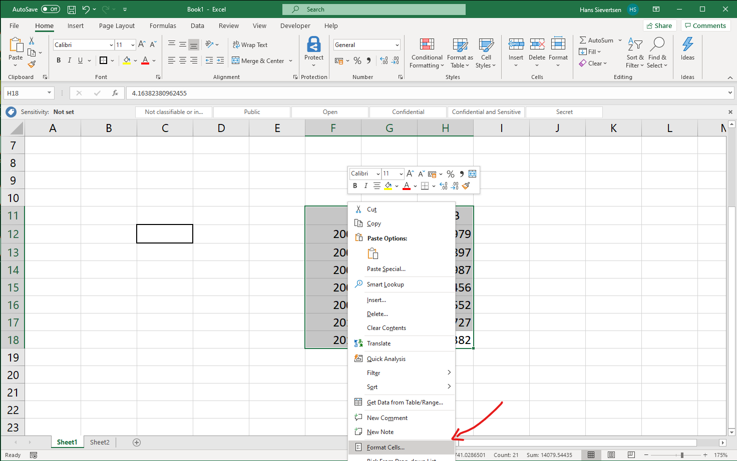
This opens a menu where we can change aspects of the cells.

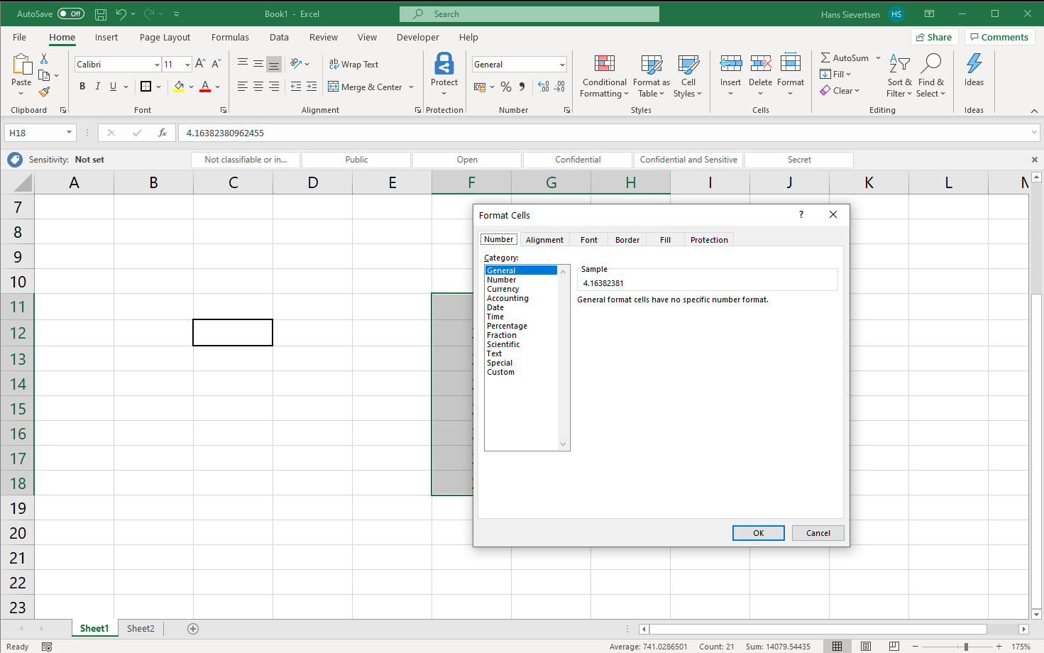
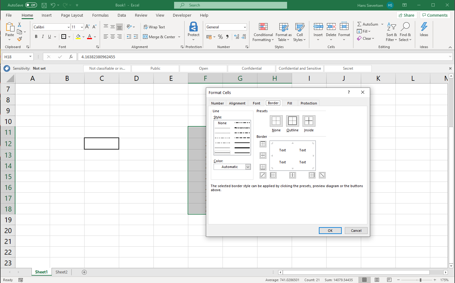
Let’s jump to the Border tab.

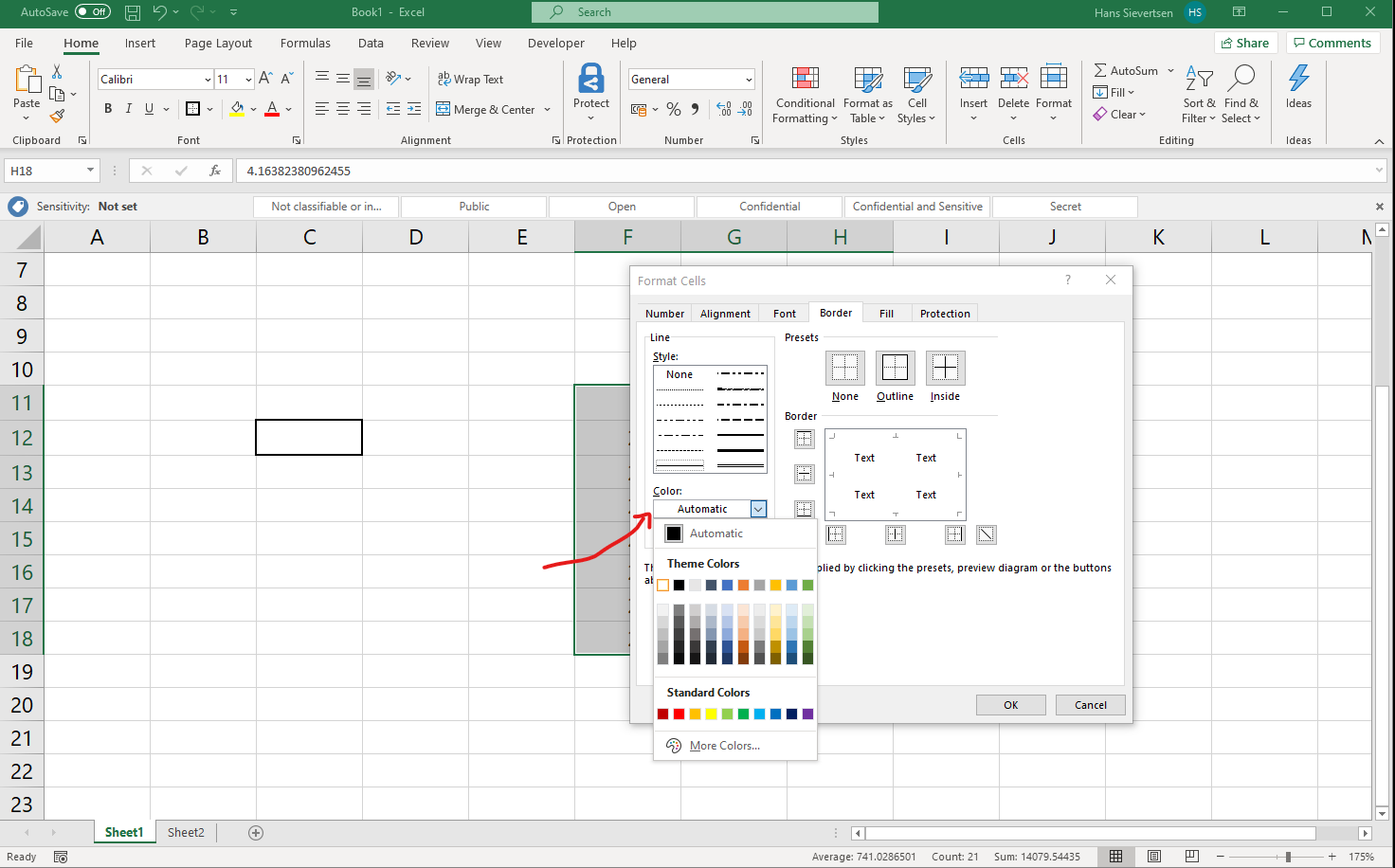
In the Color we select “White”.

We then select all the borders we want to have the new setting (the white color). In this example we select both inside and outside. Click OK to to confirm our changes.

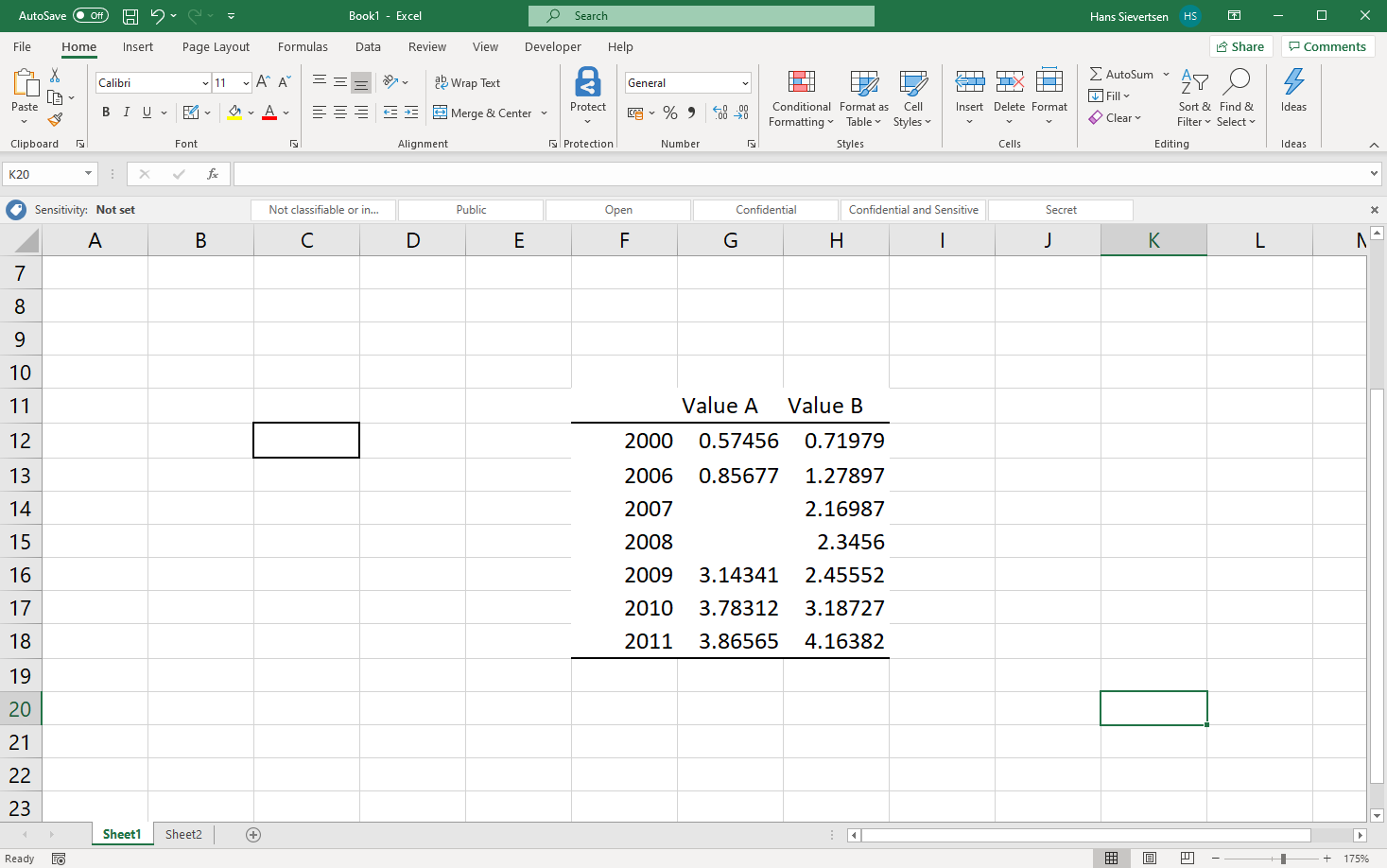
The image below shows the outcome of setting all borders in the selected area to white. The thin grey lines have disappeared! They are overwritten by the solid white lines.

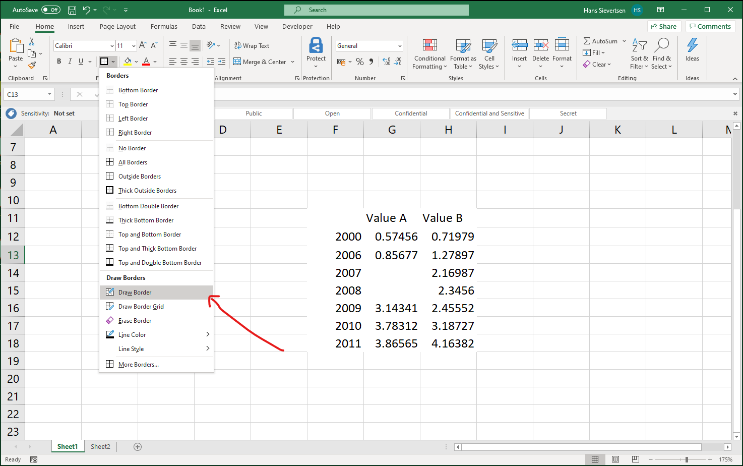
We can also change the borders manually by selecting the “Draw Border” menu as shown below.

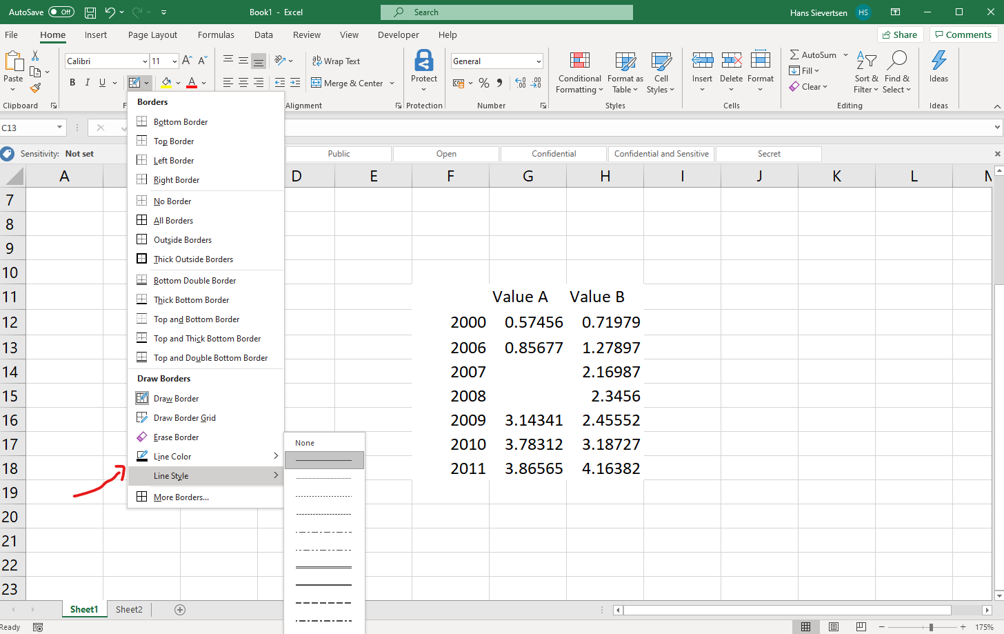
When drawing the border we can change the line type and color in the lower part of the menu.

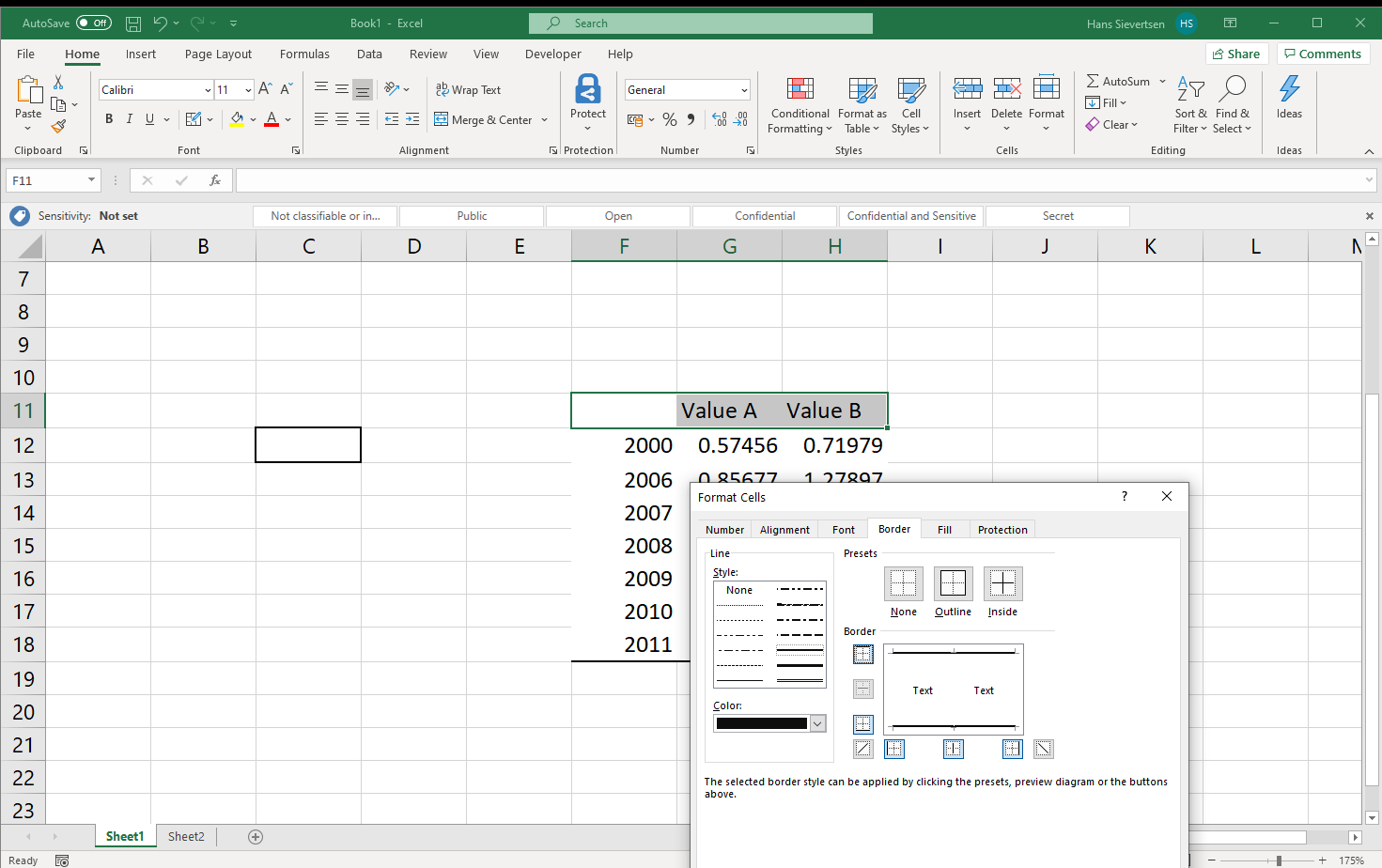
Let’s return to our initial approach and let’s select the data area again, but this time we exclude the top row in our selection.

We return to the “Format Cells” and “Border” menu. But this time we select black, and only the upper and lower border.

After we click OK the table looks like below. We’ve separated the data titles from the actual data using solid black lines.

We now repeat the process on the area with the section including the titles to add a solid top border.

Value alignment and appearance

Let’s now adjust the apperance of the values in the table. We select just the cells that contain the values as shown below.

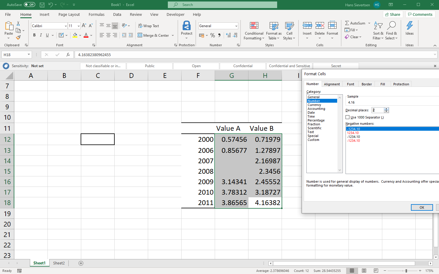
In the “Format Cells” menu we now focus on the “Number” tab. We set the “Category” to “Number”. We set the number of decimal points to 2.

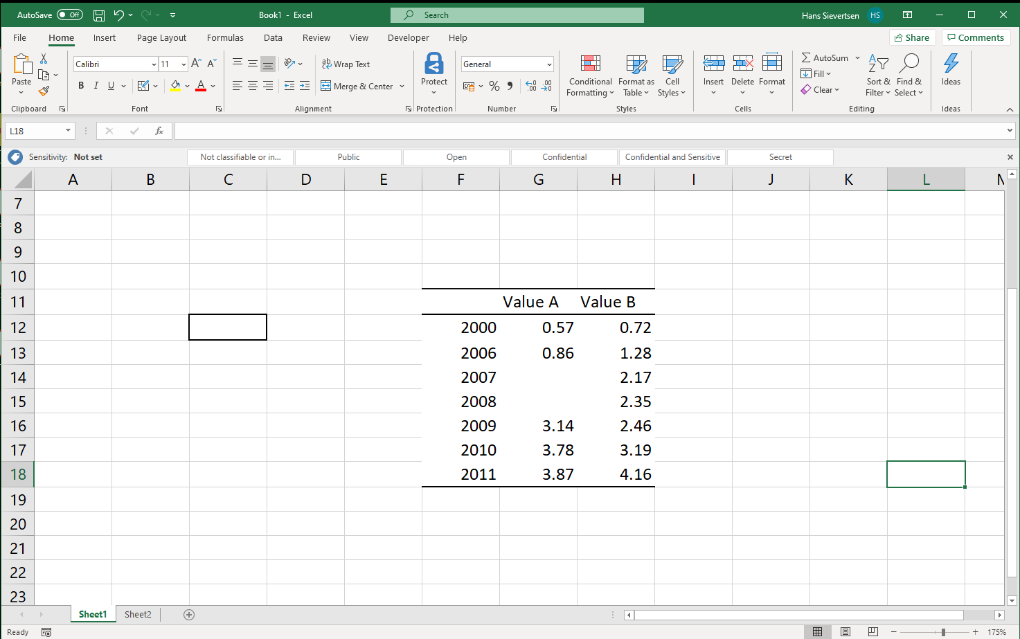
Great! All values are now shown with only two decimal points. This is much easier to read! (Note that there is also a shortcut for changing the number of decimal points directly in the ribbon).

Next, we select the same cells again and change the alignment to center the values.

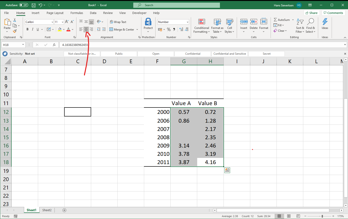
Finally, we left-align the year column. The table looks quite good!

5.2 Merging and wrapping cells

Merging cells

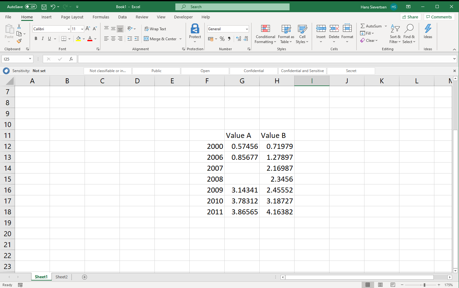
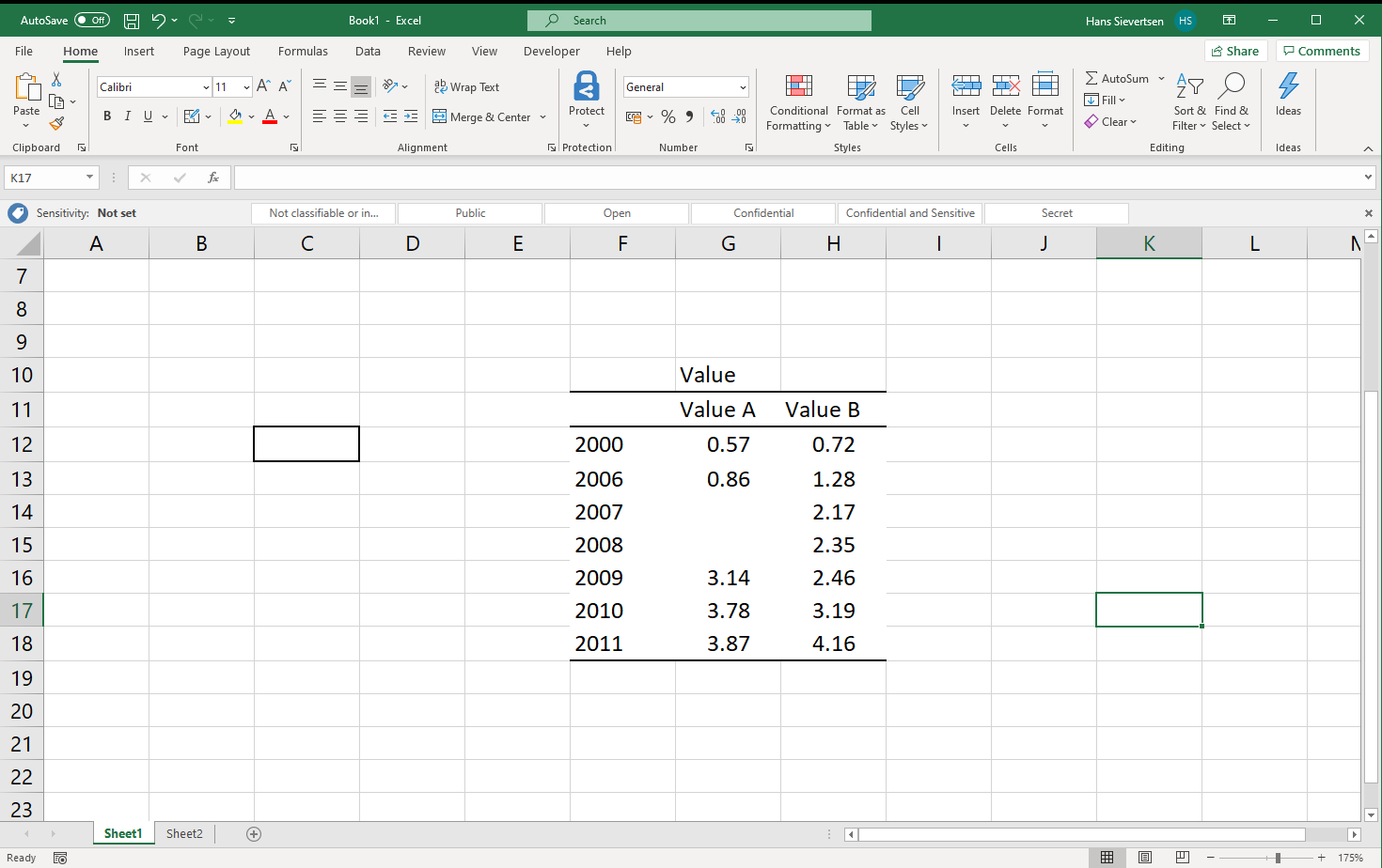
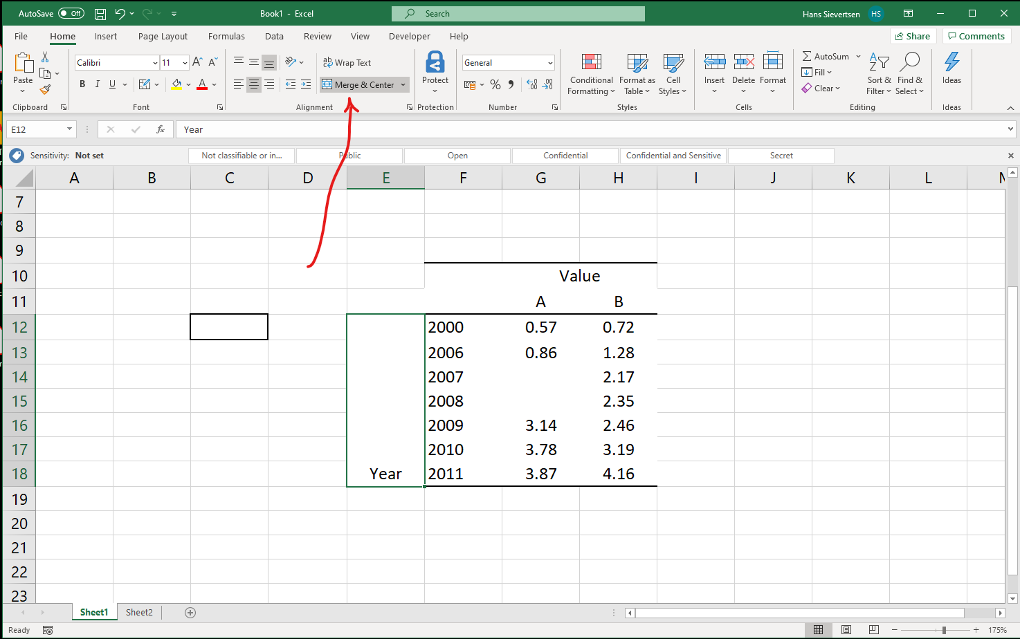
It is a bit inefficient that we repeat the word “Value” in the column headers of our table. Let us change that. First we add another general header to the columns by entering “Value” in cell G10:

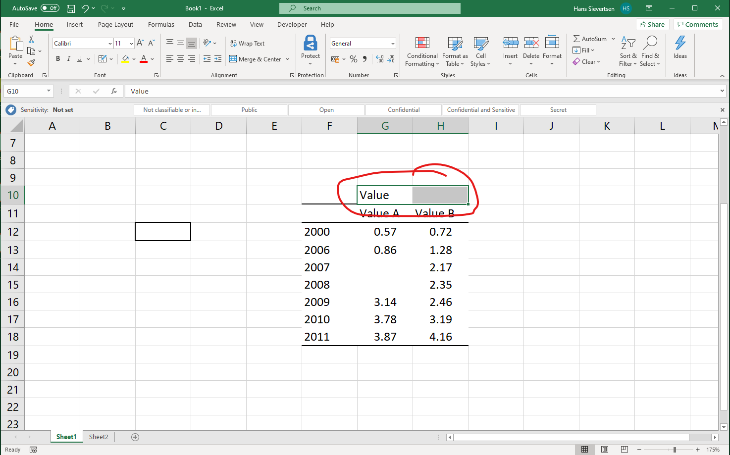
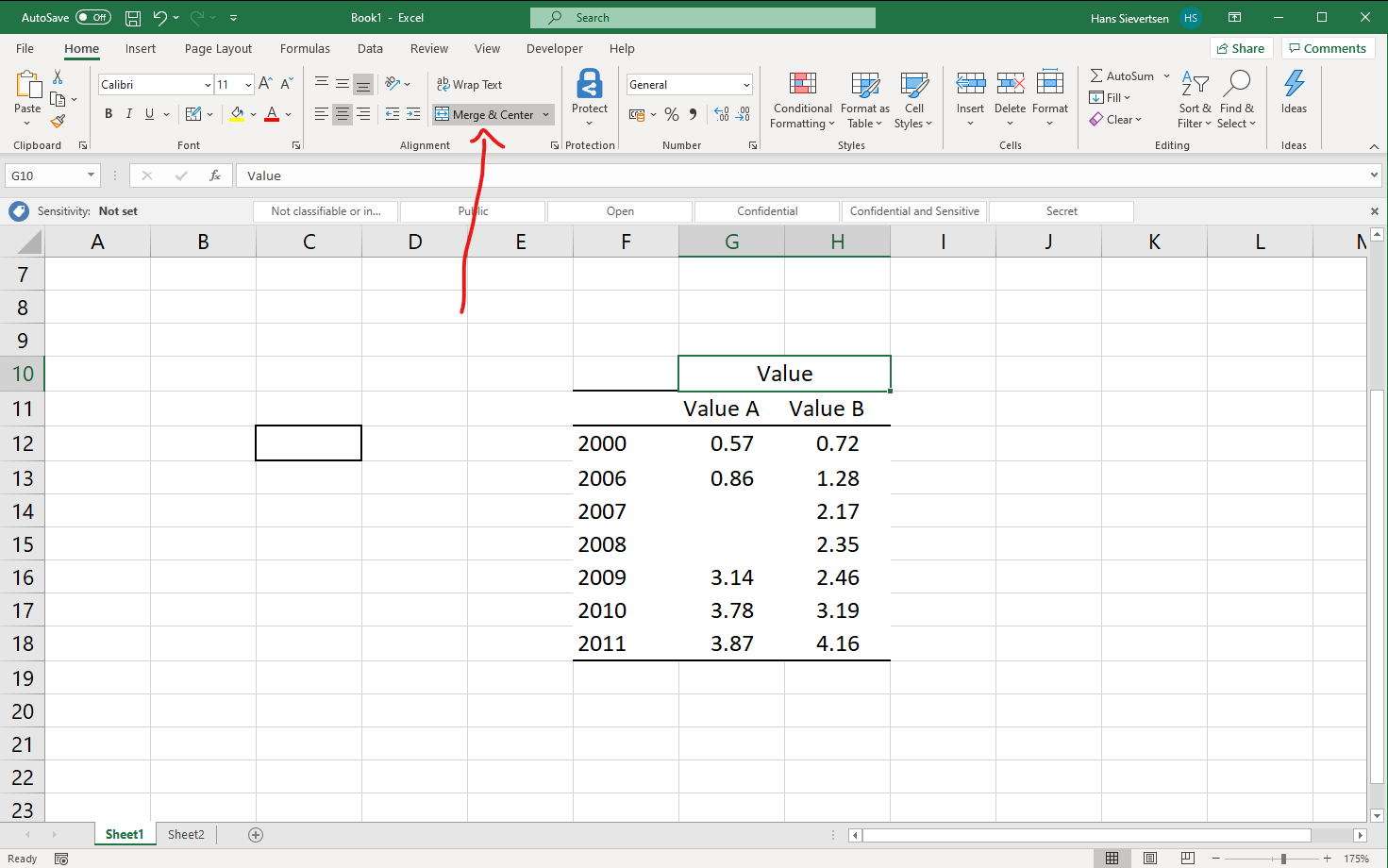
Next we select both cell G10 and cell H10. Having selected these two cells we click on “Merge & Center” as shown below. This merges the two cells and centers the title!

We repeat the process from above to modify the borders in the column title section.

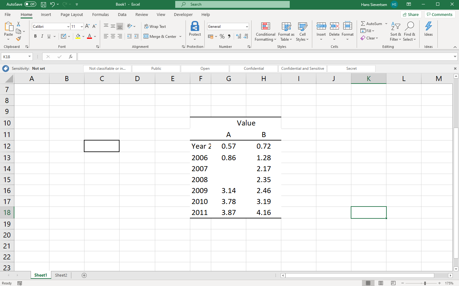
Finally, we remove the the “Value” from cells G11 and H12. We center align the text in these cells and voila. Our table looks like the one below. The advantage of merging the cells is that we can create titles that cover ceveral cells.

Text wrapping

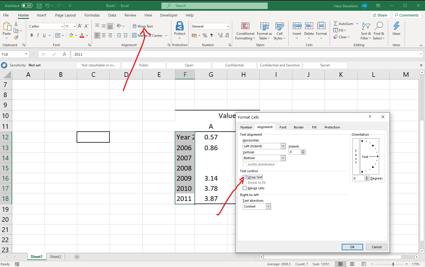
What if there is insufficient space to show all the column content as in the example below where cell F12 contains more content that we can see.

One solution is to make the cell wider. An alternative solution is to allow the text to wrap across rows. Simply select the cell and click “Wrap text”. This can be done directly in the ribbon (under Home Tab) or in the Format Cells menu, as shown below.

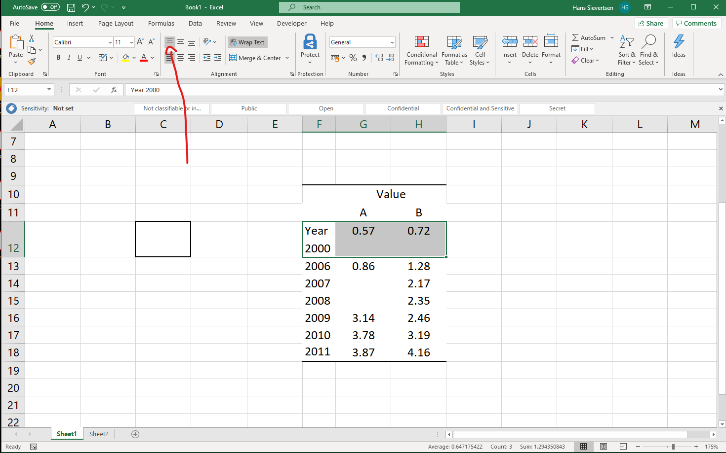
As a result, see below, the row 12 is now heigher than the other cells.

We can modify the vertical adjustment of text in a cell (either in the Format cells menu or) in the ribbon a shown below.

Text orientation

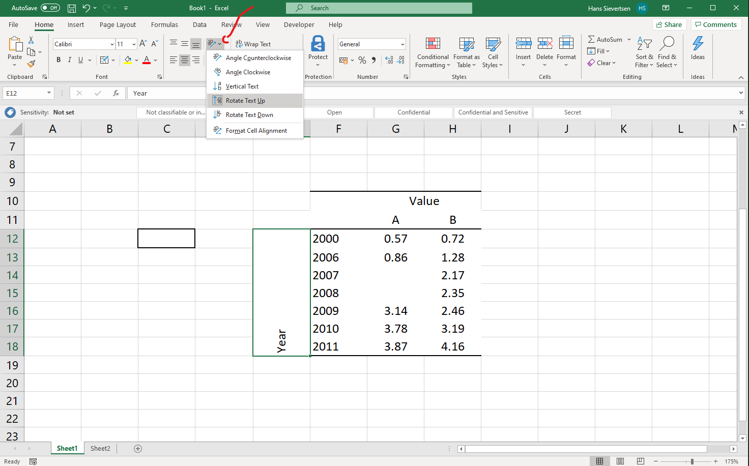
We can also merge cells vertically as shown below.

In a case like the example above, we might want to change the orientation of the text not be horisontal, but be rotated. Select the cells where want to to change the text orientation and click on the text-orientation icon in the ribbon (the Home Tab ribbon) as shown below. This option is also available in the Format Cells menu.

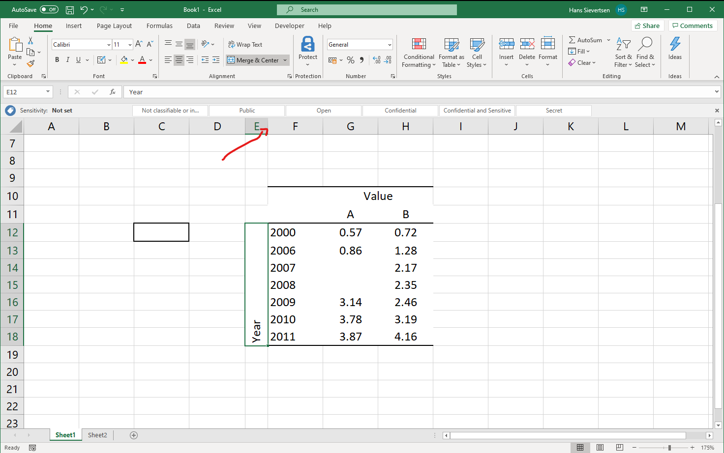
Cell (and row) width

We can change the width of row by clicking on the line separating two columns and dragging the mouse in a direction as shown below. The same goes for rows!

5.3 The format painter

What if we’ve finished formatting cells, but we accidentally forgot to select cells to included. Do we have to repeat everything on these cells? No! We can use the formatting paint. Here is how it works.

1. Select the cells that have the right format that we want to apply on other cells.

2. Click on the “Format painter” icon in the Home Tab Ribbon as shown below.

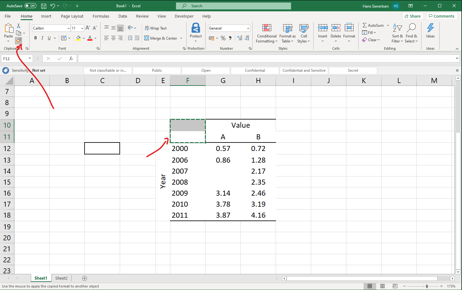
3. Select all the cells where you want to apply the format.

Voila!