Roy 1951: Some Thoughts on the Distribution of Earnings

A Reading Companion with R Simulations

library(tidyverse)
library(MASS)
library(patchwork)

# Set seed for reproducibility
set.seed(1951)

# Number of workers in simulations
n <- 10000

# Core simulation function we'll use throughout
simulate_roy <- function(n, rho, sigma_h = 0.3, sigma_f = 0.8,
                         mu_h = 4, mu_f = 3, p_r = 1, p_f = 3) {
  Sigma <- matrix(c(
    sigma_h^2, rho * sigma_h * sigma_f,
    rho * sigma_h * sigma_f, sigma_f^2
  ), nrow = 2)

  log_out <- mvrnorm(n, mu = c(mu_h, mu_f), Sigma = Sigma)

  tibble(
    log_hunt = log_out[, 1],
    log_fish = log_out[, 2],
    output_hunt = exp(log_hunt),
    output_fish = exp(log_fish),
    earnings_hunt = p_r * exp(log_hunt),
    earnings_fish = p_f * exp(log_fish),
    chosen = if_else(earnings_fish > earnings_hunt, "Fishing", "Hunting"),
    actual_earnings = pmax(earnings_hunt, earnings_fish)
  )
}

---

Section I: Introduction

Roy begins by presenting the foundational insight that individual output results from many random influences operating proportionately rather than absolutely. This leads naturally to log-normal distributions.

The Paper Begins

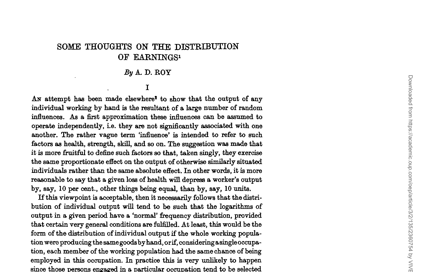
Key insight: Random factors like health, strength, and skill affect output proportionately (e.g., illness reduces output by 10%, not by 10 units). This multiplicative effect implies that log output is normally distributed.

The Selection Problem

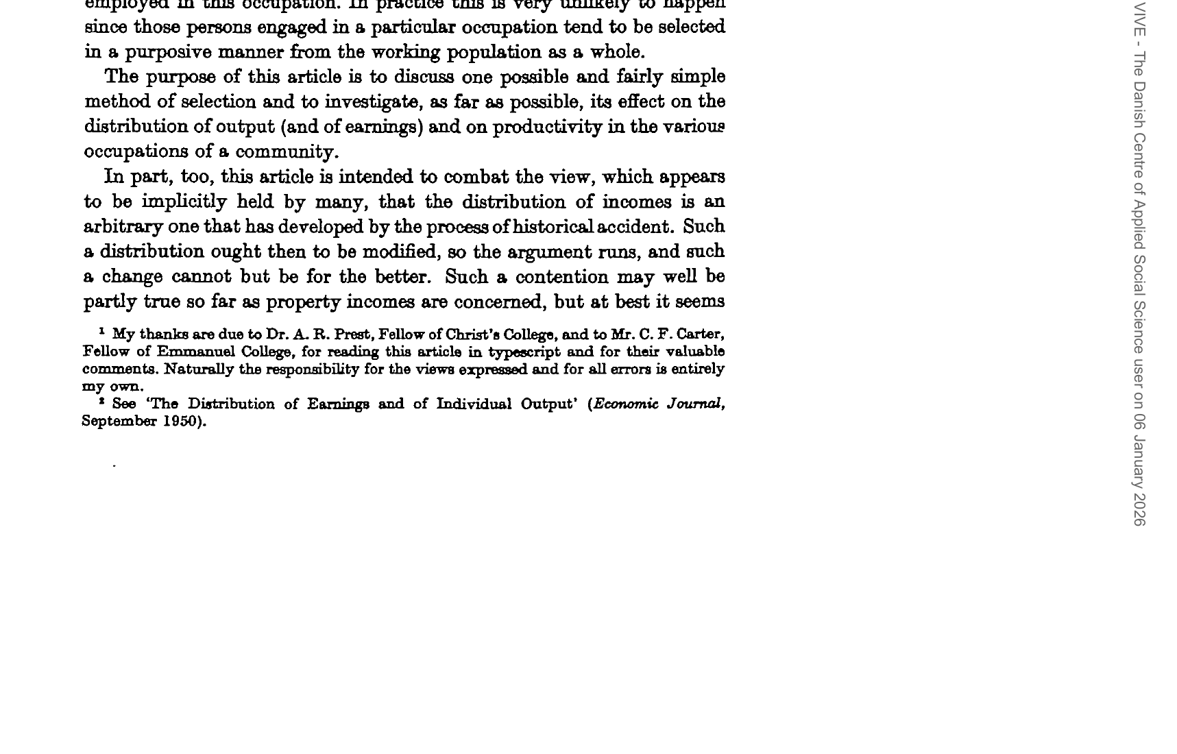
Roy’s main argument: the distribution of earnings is not arbitrary but depends on “real” factors—the distribution of human skills and technology—not merely on prices or social conventions.

---

Roy’s Main Thesis

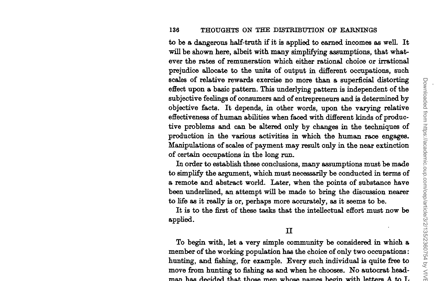
The core claim: Whatever prices are set for different occupations’ outputs, they can only superficially distort an underlying pattern determined by objective facts—the relative effectiveness of human abilities across different productive activities.

---

Section II: The Two-Occupation Model

Roy introduces a simple village economy with two occupations: hunting (rabbits) and fishing (trout).

The Setup

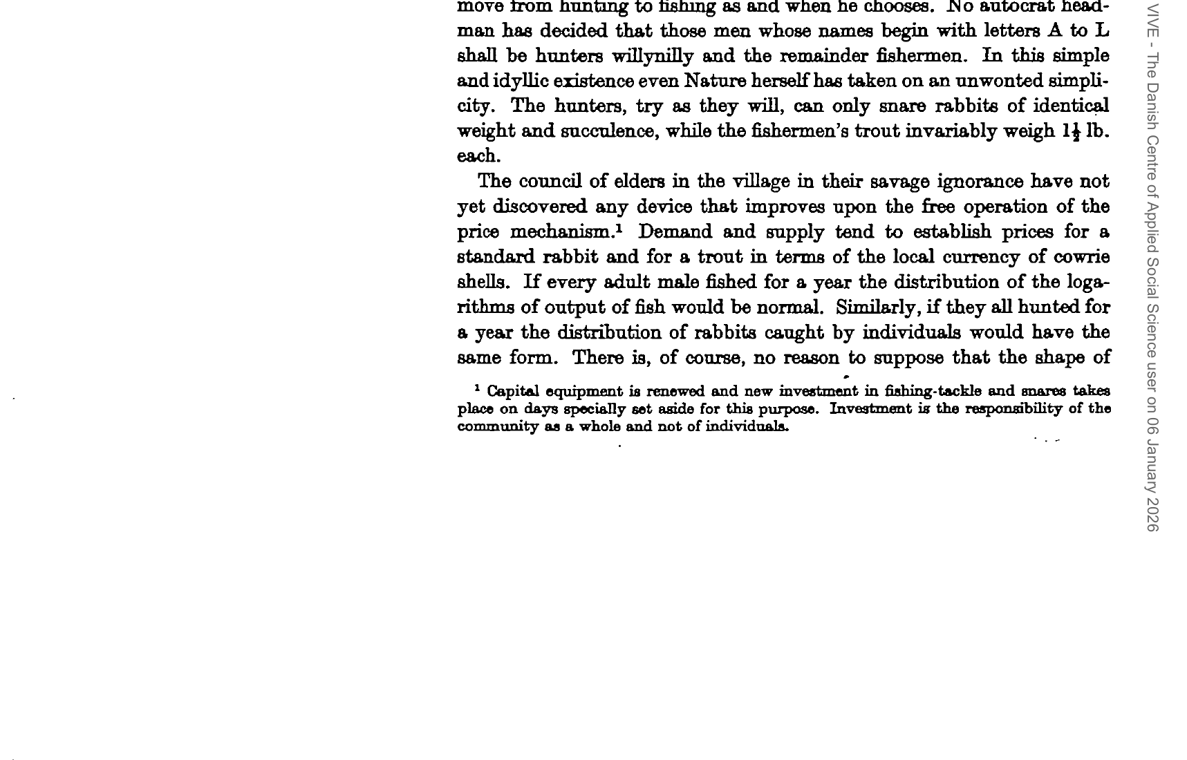
Key assumptions:

• Free occupational choice (no central planning)
• Standardized output (identical rabbits, identical trout)
• Price mechanism operates freely
• Log-normal output distributions in both occupations

---

Concentration of Output Distributions

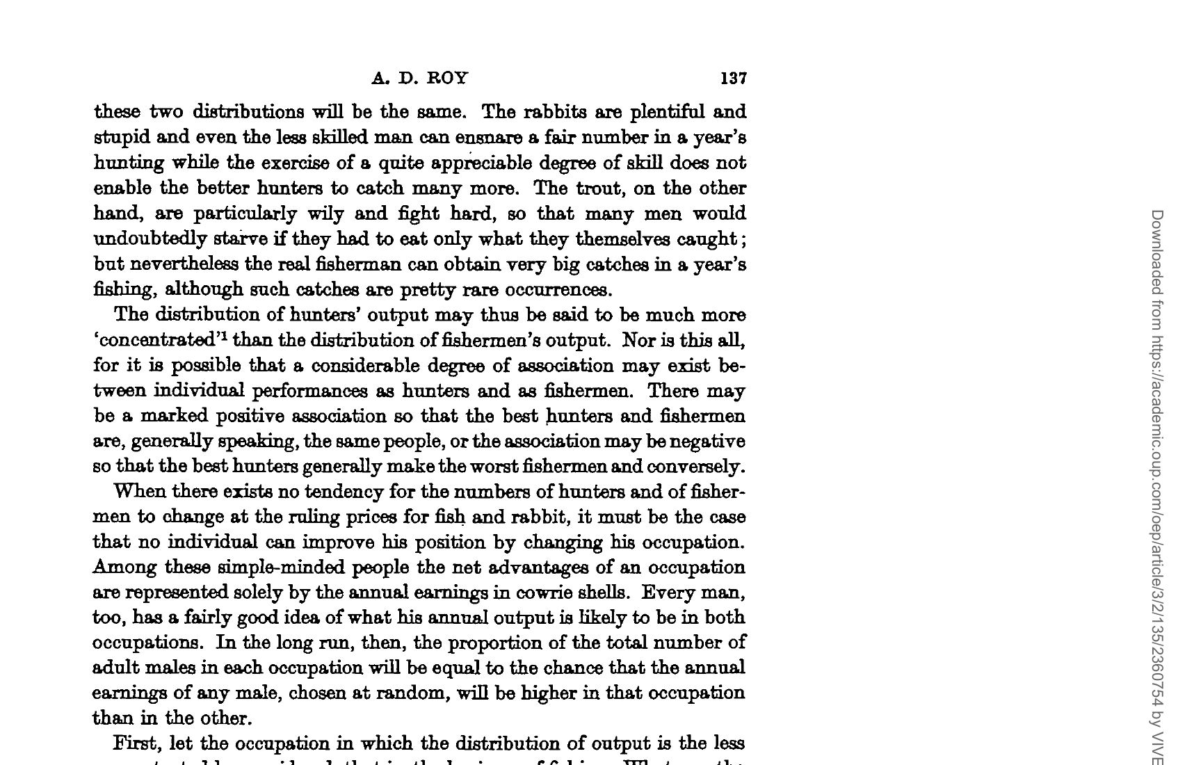
Critical distinction:

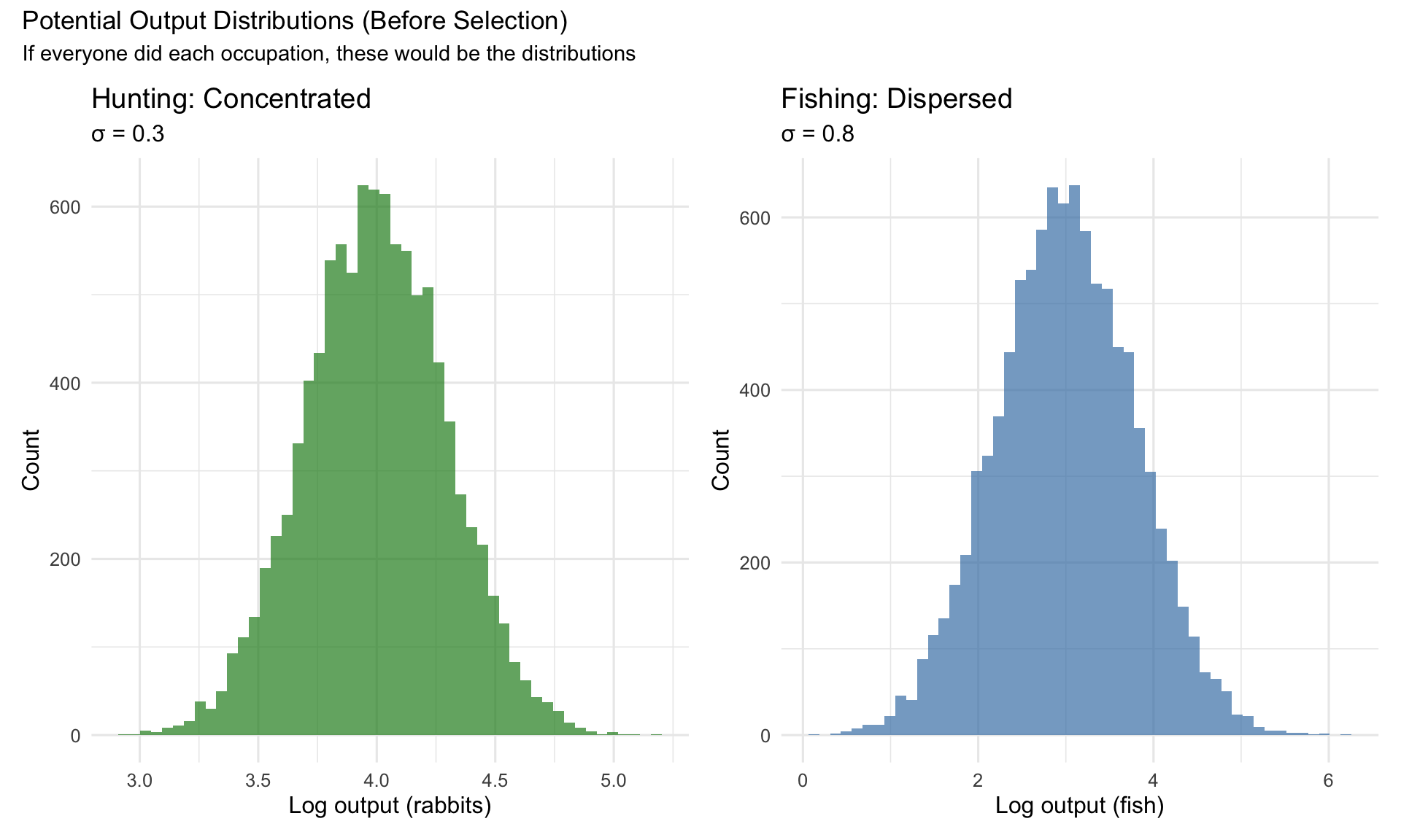
• Hunting (rabbits): Output is “concentrated” (low variance)—rabbits are “plentiful and stupid,” so even poor hunters catch a fair number, but skill doesn’t help much
• Fishing (trout): Output is “dispersed” (high variance)—trout are “particularly wily,” so unskilled fishermen catch little, but experts can have huge catches

R Simulation: The Basic Setup

Code

# Parameters matching Roy's description
mu_hunt <- 4
mu_fish <- 3
sigma_hunt <- 0.3  # Concentrated (low variance)
sigma_fish <- 0.8  # Dispersed (high variance)
rho <- 0.5

# Simulate potential outputs for entire population
set.seed(1951)
village <- simulate_roy(n, rho = rho, sigma_h = sigma_hunt, sigma_f = sigma_fish,
                        mu_h = mu_hunt, mu_f = mu_fish)

# Plot potential distributions
p1 <- ggplot(village, aes(x = log_hunt)) +
  geom_histogram(bins = 50, fill = "forestgreen", alpha = 0.7) +
  labs(x = "Log output (rabbits)", y = "Count",
       title = "Hunting: Concentrated",
       subtitle = paste0("σ = ", sigma_hunt)) +
  theme_minimal(base_size = 12)

p2 <- ggplot(village, aes(x = log_fish)) +
  geom_histogram(bins = 50, fill = "steelblue", alpha = 0.7) +
  labs(x = "Log output (fish)", y = "Count",
       title = "Fishing: Dispersed",
       subtitle = paste0("σ = ", sigma_fish)) +
  theme_minimal(base_size = 12)

p1 + p2 + plot_annotation(
  title = "Potential Output Distributions (Before Selection)",
  subtitle = "If everyone did each occupation, these would be the distributions"
)

Figure 1: Potential output distributions: Hunting is concentrated, Fishing is dispersed

---

The Selection Mechanism

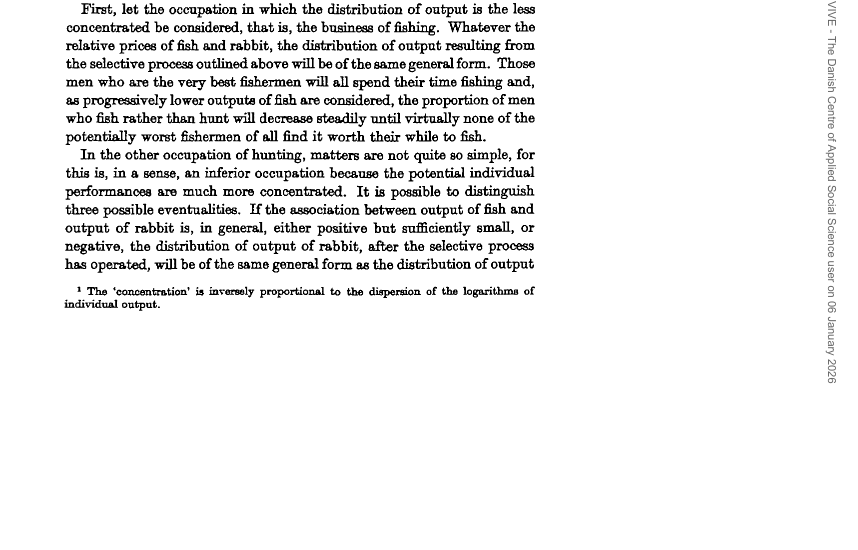
How workers choose:

• Each worker knows their potential output in both occupations
• They choose whichever pays more: \(\max(p_R \cdot Y_R, p_F \cdot Y_F)\)
• In equilibrium, no one wants to switch

Selection into fishing: The best potential fishermen will fish; as we consider lower potential outputs, fewer choose fishing.

---

Selection Effects on Distribution

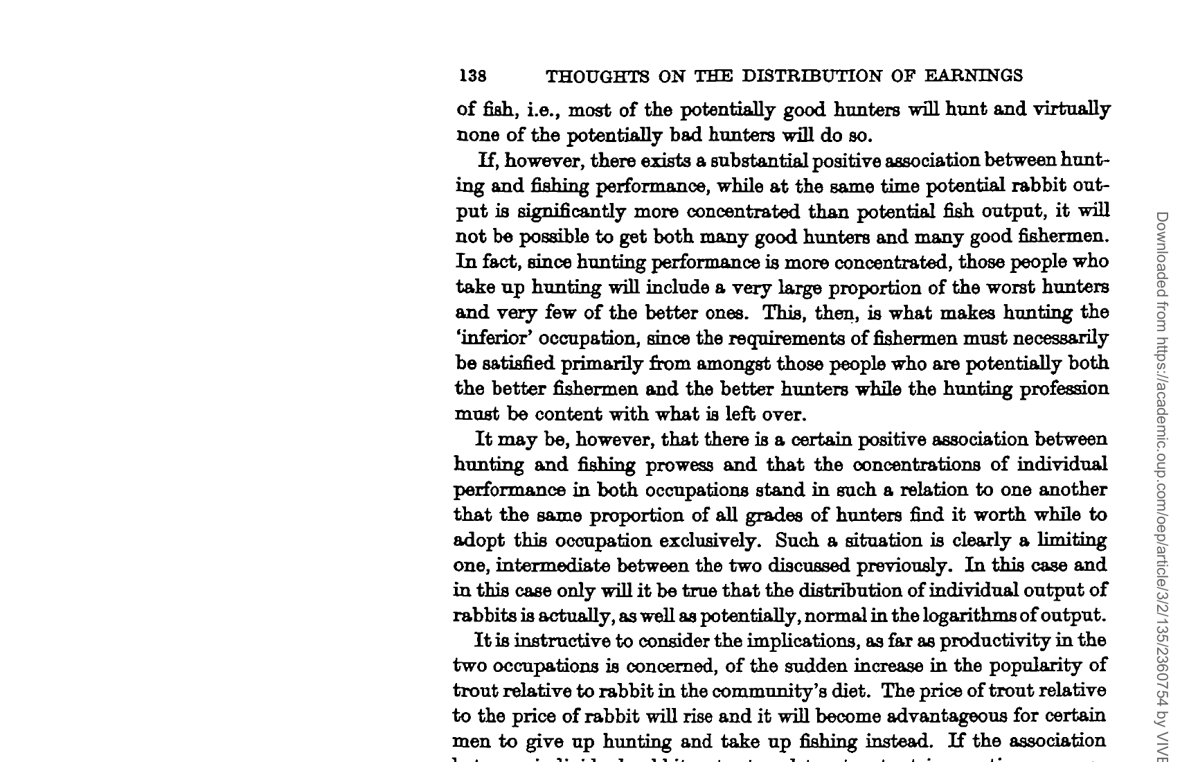
Key result: When skills are positively correlated but fishing has higher variance:

• Good hunters who are even better fishermen → fish
• This can make hunting an “inferior” occupation populated by those who are mediocre at both

R Simulation: The Selection Process

Code

# Price ratio
p_rabbit <- 1
p_fish <- 3

# Selection boundary: p_f * Y_f = p_r * Y_r
# In logs: log(Y_f) = log(Y_r) + log(p_r/p_f)
boundary_intercept <- log(p_rabbit / p_fish)

ggplot(village, aes(x = log_hunt, y = log_fish, color = chosen)) +
  geom_point(alpha = 0.3, size = 0.8) +
  geom_abline(intercept = boundary_intercept, slope = 1,
              linetype = "dashed", linewidth = 1.2) +
  scale_color_manual(values = c("Fishing" = "steelblue", "Hunting" = "forestgreen")) +
  labs(
    x = "Log potential hunting output",
    y = "Log potential fishing output",
    color = "Chosen\nOccupation",
    title = "Occupational Self-Selection",
    subtitle = "Workers choose the occupation that maximizes their earnings"
  ) +
  theme_minimal(base_size = 12) +
  annotate("text", x = 3.3, y = 5.2, label = "Fish", size = 5, fontface = "bold", color = "steelblue") +
  annotate("text", x = 4.7, y = 1.8, label = "Hunt", size = 5, fontface = "bold", color = "forestgreen") +
  annotate("text", x = 4.5, y = 3.8, label = "Selection\nboundary", size = 3, color = "black")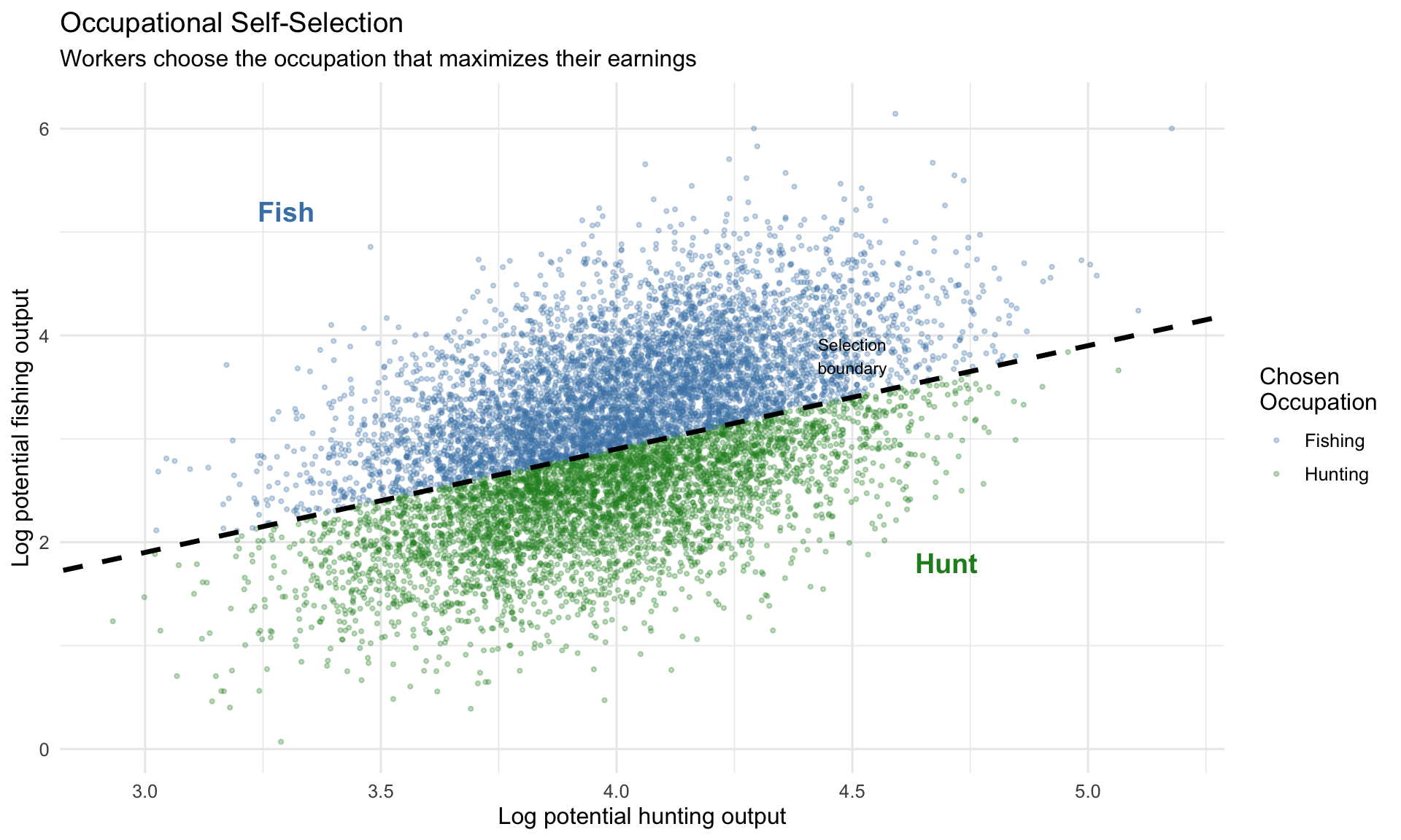

Figure 2: Workers select based on comparative advantage in earnings

Code

# Show who actually chose each occupation
village_long <- village |>
  pivot_longer(cols = c(output_hunt, output_fish),
               names_to = "occupation_type", values_to = "potential_output") |>
  mutate(
    occupation_type = if_else(occupation_type == "output_hunt", "Hunting", "Fishing"),
    is_chosen = chosen == occupation_type
  )

ggplot(village_long, aes(x = log(potential_output), fill = is_chosen)) +
  geom_histogram(bins = 50, alpha = 0.7, position = "identity") +
  facet_wrap(~occupation_type) +
  scale_fill_manual(
    values = c("TRUE" = "darkblue", "FALSE" = "gray70"),
    labels = c("TRUE" = "Actually in this occupation", "FALSE" = "Chose the other")
  ) +
  labs(
    x = "Log output",
    y = "Count",
    fill = "",
    title = "Potential vs. Observed: Selection Creates Truncation",
    subtitle = "Best fishermen fish; hunting gets a more mixed ability distribution"
  ) +
  theme_minimal(base_size = 12)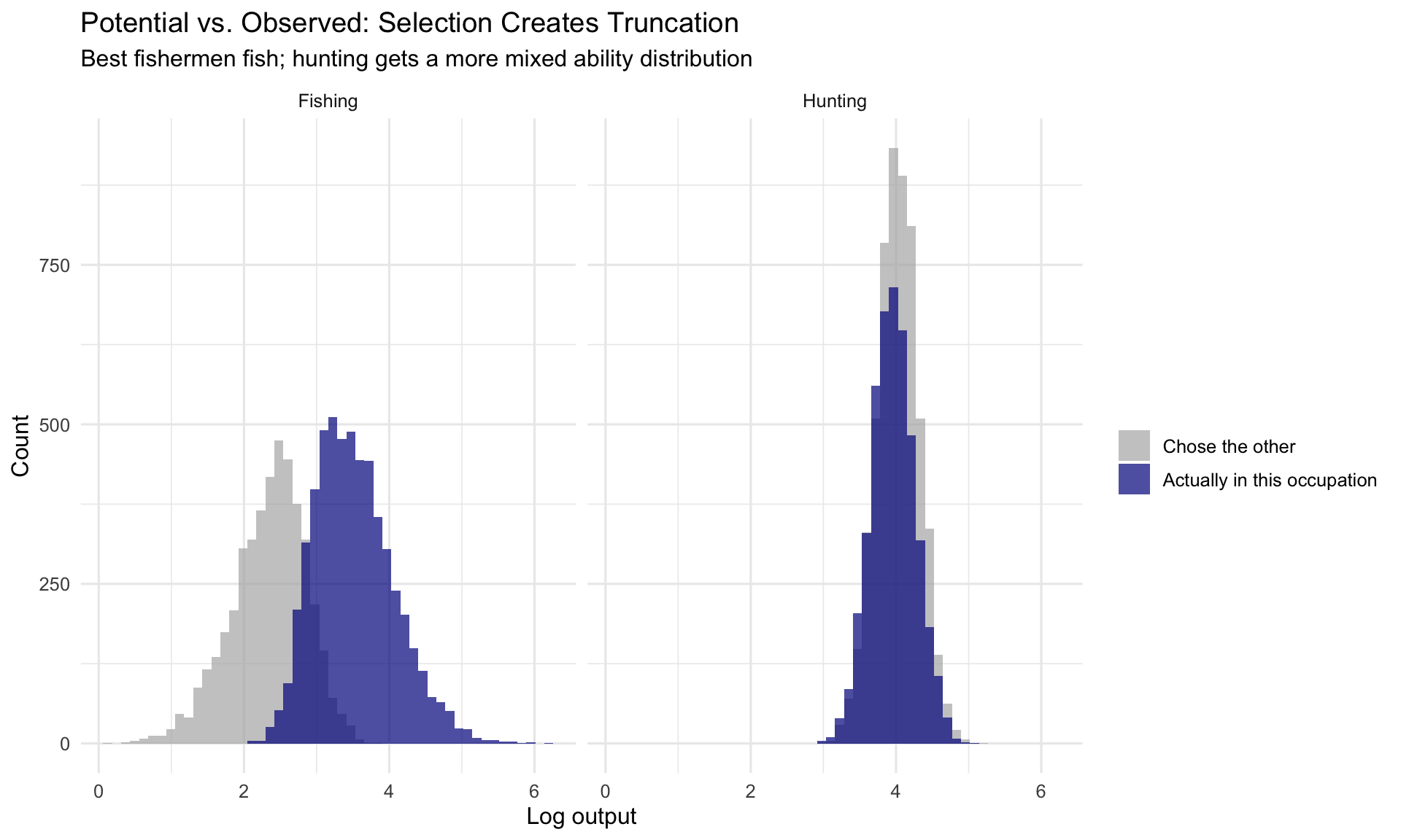

Figure 3: Selection skews observed output distributions

---

Productivity Effects of Demand Changes

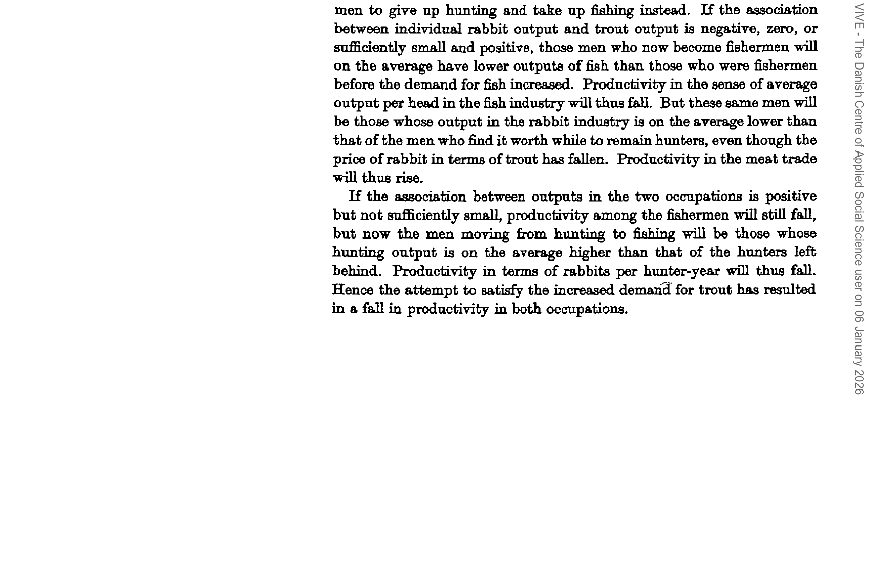
Roy’s insight on productivity:

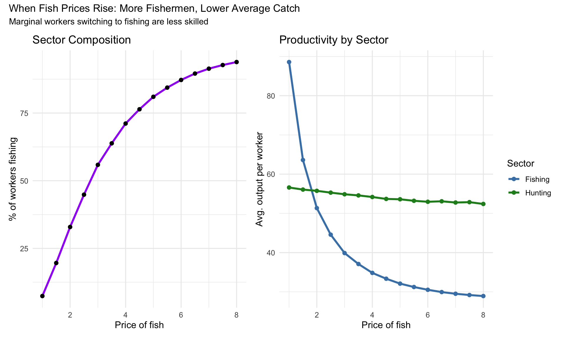
When demand for fish rises (price of fish increases):

• More workers switch to fishing
• The marginal switchers are worse at fishing → fishing productivity falls
• But they were also below-average hunters → hunting productivity rises

This is a profound result: trying to get more of something can reduce average quality!

R Simulation: Demand Shifts and Productivity

Code

# Analyze productivity at different fish prices
analyze_productivity <- function(p_fish_vec, village_data) {
  map_dfr(p_fish_vec, function(p_f) {
    earnings_hunt <- 1 * village_data$output_hunt
    earnings_fish <- p_f * village_data$output_fish

    is_fisher <- earnings_fish > earnings_hunt

    tibble(
      p_fish = p_f,
      pct_fishers = mean(is_fisher) * 100,
      avg_fish_output = mean(village_data$output_fish[is_fisher]),
      avg_hunt_output = mean(village_data$output_hunt[!is_fisher])
    )
  })
}

price_analysis <- analyze_productivity(seq(1, 8, by = 0.5), village)

p1 <- ggplot(price_analysis, aes(x = p_fish, y = pct_fishers)) +
  geom_line(linewidth = 1.2, color = "purple") +
  geom_point(size = 2) +
  labs(x = "Price of fish", y = "% of workers fishing",
       title = "Sector Composition") +
  theme_minimal(base_size = 12)

p2 <- price_analysis |>
  pivot_longer(cols = c(avg_fish_output, avg_hunt_output),
               names_to = "sector", values_to = "productivity") |>
  mutate(sector = if_else(sector == "avg_fish_output", "Fishing", "Hunting")) |>
  ggplot(aes(x = p_fish, y = productivity, color = sector)) +
  geom_line(linewidth = 1.2) +
  geom_point(size = 2) +
  scale_color_manual(values = c("Fishing" = "steelblue", "Hunting" = "forestgreen")) +
  labs(x = "Price of fish", y = "Avg. output per worker", color = "Sector",
       title = "Productivity by Sector") +
  theme_minimal(base_size = 12)

p1 + p2 + plot_annotation(
  title = "When Fish Prices Rise: More Fishermen, Lower Average Catch",
  subtitle = "Marginal workers switching to fishing are less skilled"
)

Figure 4: How price changes affect sector productivity

---

The Limiting Case

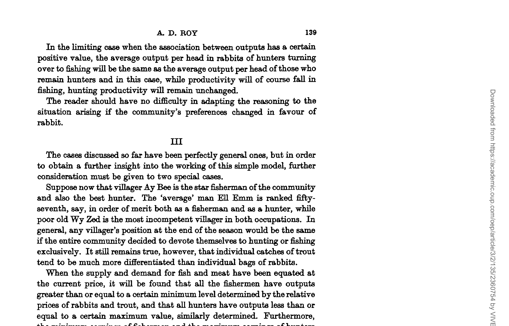
When the correlation has a certain positive value, productivity among hunters remains unchanged even as workers switch to fishing. This is a knife-edge case.

---

Section III: Special Cases

Roy now examines two illuminating special cases.

Perfect Positive Correlation: “Ay Bee is Champion”

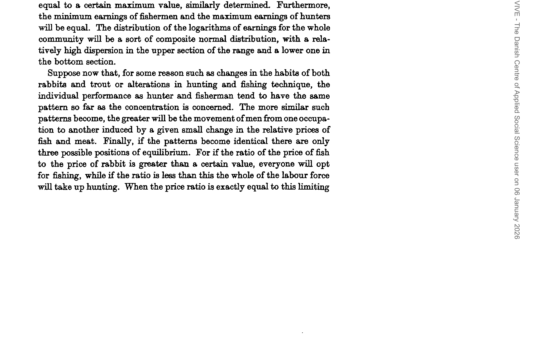
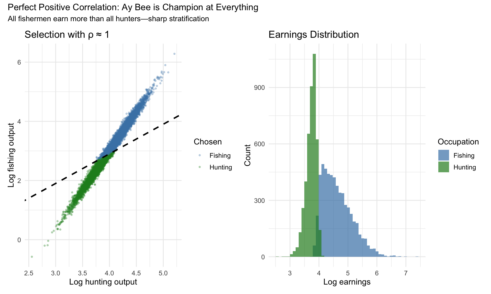
Case 1 (ρ = 1): Villager “Ay Bee” is the best at everything. Rankings are identical across occupations: best fisherman = best hunter. “Ell Emm” is 57th in both. Poor “Wy Zed” is worst at both.

Result: Sharp earnings stratification—all fishermen earn more than all hunters.

R Simulation: Perfect Positive Correlation

Code

village_pos <- simulate_roy(n, rho = 0.99)

p1 <- ggplot(village_pos, aes(x = log_hunt, y = log_fish, color = chosen)) +
  geom_point(alpha = 0.3, size = 0.8) +
  geom_abline(intercept = log(1/3), slope = 1, linetype = "dashed", linewidth = 1) +
  scale_color_manual(values = c("Fishing" = "steelblue", "Hunting" = "forestgreen")) +
  labs(x = "Log hunting output", y = "Log fishing output", color = "Chosen",
       title = "Selection with ρ ≈ 1") +
  theme_minimal(base_size = 12)

p2 <- ggplot(village_pos, aes(x = log(actual_earnings), fill = chosen)) +
  geom_histogram(bins = 50, alpha = 0.7, position = "identity") +
  scale_fill_manual(values = c("Fishing" = "steelblue", "Hunting" = "forestgreen")) +
  labs(x = "Log earnings", y = "Count", fill = "Occupation",
       title = "Earnings Distribution") +
  theme_minimal(base_size = 12)

p1 + p2 + plot_annotation(
  title = "Perfect Positive Correlation: Ay Bee is Champion at Everything",
  subtitle = "All fishermen earn more than all hunters—sharp stratification"
)

Figure 5: With ρ ≈ 1: Sharp ability-based sorting into occupations

---

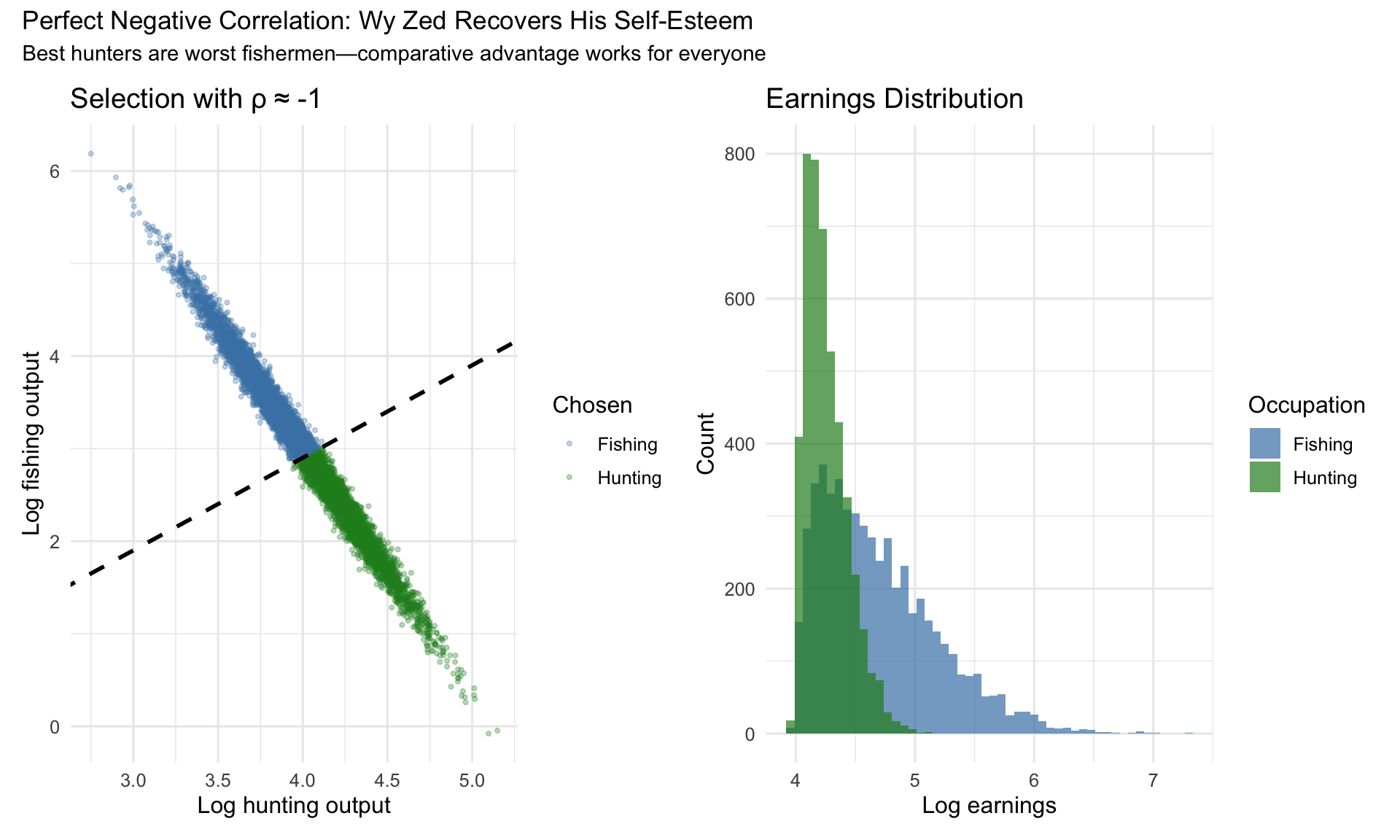
Perfect Negative Correlation: “Wy Zed Recovers His Self-Esteem”

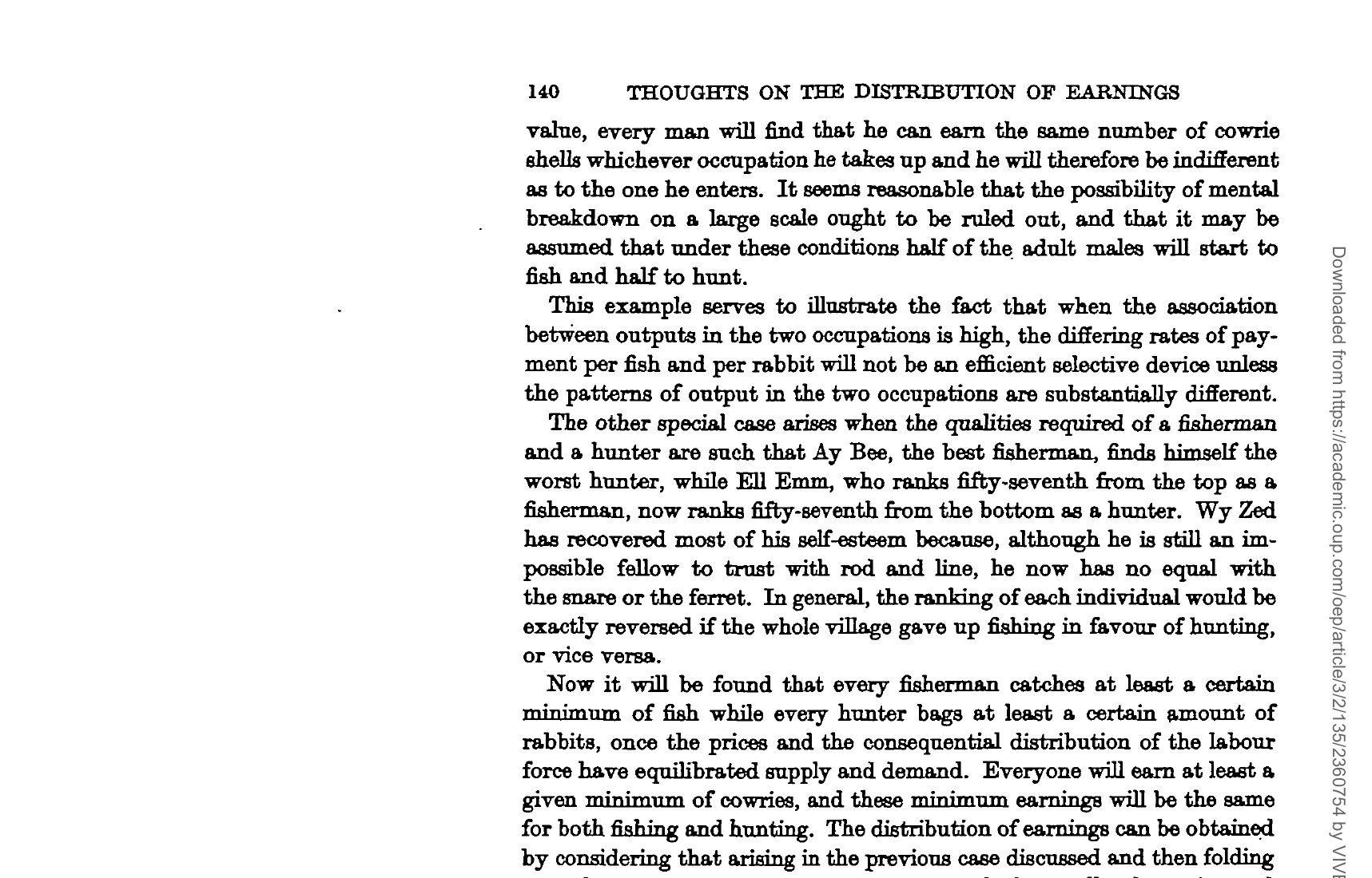
Case 2 (ρ = -1): “Ay Bee” is the best fisherman but the worst hunter. “Wy Zed” excels at hunting but is hopeless at fishing. Rankings are exactly reversed.

Result: Everyone specializes in their comparative advantage. Earnings distributions overlap—hunters and fishermen both include high and low earners.

R Simulation: Perfect Negative Correlation

Code

village_neg <- simulate_roy(n, rho = -0.99)

p1 <- ggplot(village_neg, aes(x = log_hunt, y = log_fish, color = chosen)) +
  geom_point(alpha = 0.3, size = 0.8) +
  geom_abline(intercept = log(1/3), slope = 1, linetype = "dashed", linewidth = 1) +
  scale_color_manual(values = c("Fishing" = "steelblue", "Hunting" = "forestgreen")) +
  labs(x = "Log hunting output", y = "Log fishing output", color = "Chosen",
       title = "Selection with ρ ≈ -1") +
  theme_minimal(base_size = 12)

p2 <- ggplot(village_neg, aes(x = log(actual_earnings), fill = chosen)) +
  geom_histogram(bins = 50, alpha = 0.7, position = "identity") +
  scale_fill_manual(values = c("Fishing" = "steelblue", "Hunting" = "forestgreen")) +
  labs(x = "Log earnings", y = "Count", fill = "Occupation",
       title = "Earnings Distribution") +
  theme_minimal(base_size = 12)

p1 + p2 + plot_annotation(
  title = "Perfect Negative Correlation: Wy Zed Recovers His Self-Esteem",
  subtitle = "Best hunters are worst fishermen—comparative advantage works for everyone"
)

Figure 6: With ρ ≈ -1: Everyone specializes in their strength

---

The “Superior” Occupation

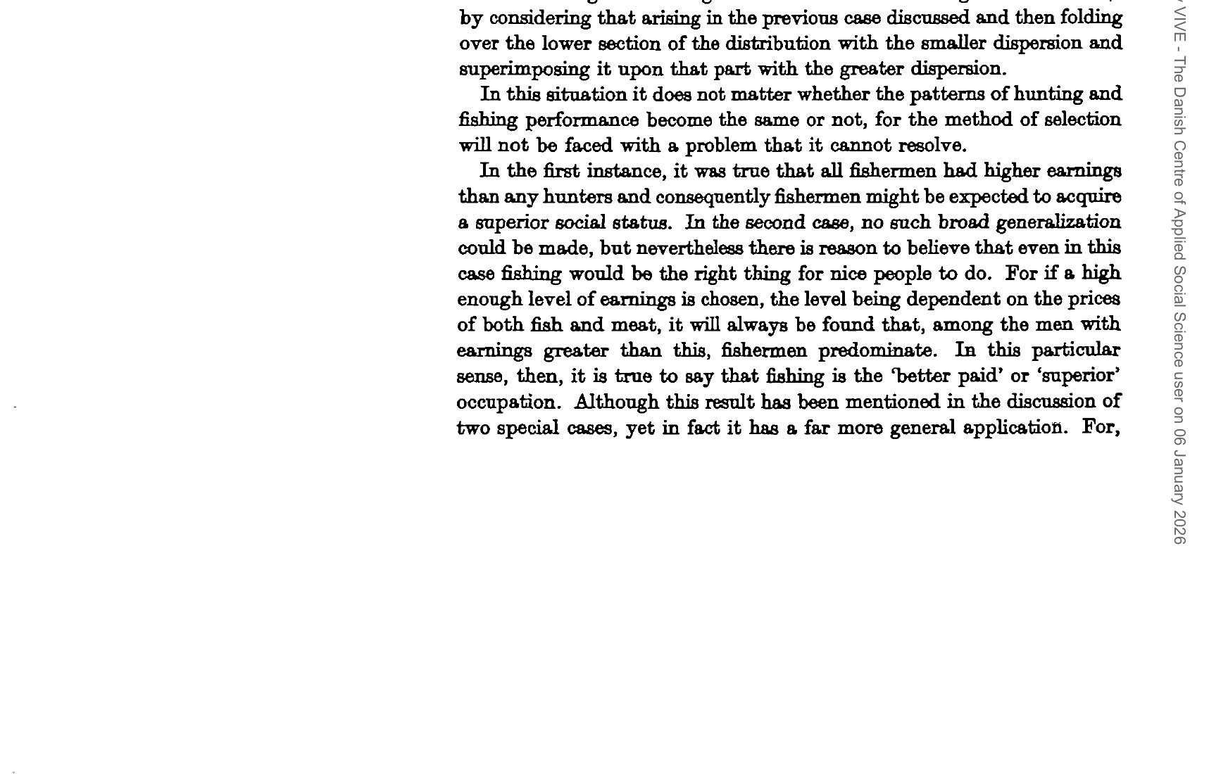
Key result: Regardless of correlation, fishing is always the “superior” occupation in the sense that at high enough earnings levels, fishermen predominate. This is because fishing has higher variance—the very top earners will be fishermen.

R Simulation: Comparing Across Correlations

Code

# Simulate across correlations
rhos <- c(-0.8, 0, 0.5, 0.95)
all_villages <- map_dfr(rhos, ~simulate_roy(n, rho = .x) |> mutate(rho = .x))

all_villages |>
  mutate(rho_label = paste0("ρ = ", rho)) |>
  ggplot(aes(x = log(actual_earnings), fill = chosen)) +
  geom_histogram(bins = 40, alpha = 0.7, position = "identity") +
  facet_wrap(~rho_label, ncol = 2) +
  scale_fill_manual(values = c("Fishing" = "steelblue", "Hunting" = "forestgreen")) +
  labs(x = "Log earnings", y = "Count", fill = "Occupation",
       title = "Earnings Distributions Under Different Skill Correlations",
       subtitle = "Higher positive correlation → sharper stratification; negative correlation → more overlap") +
  theme_minimal(base_size = 12)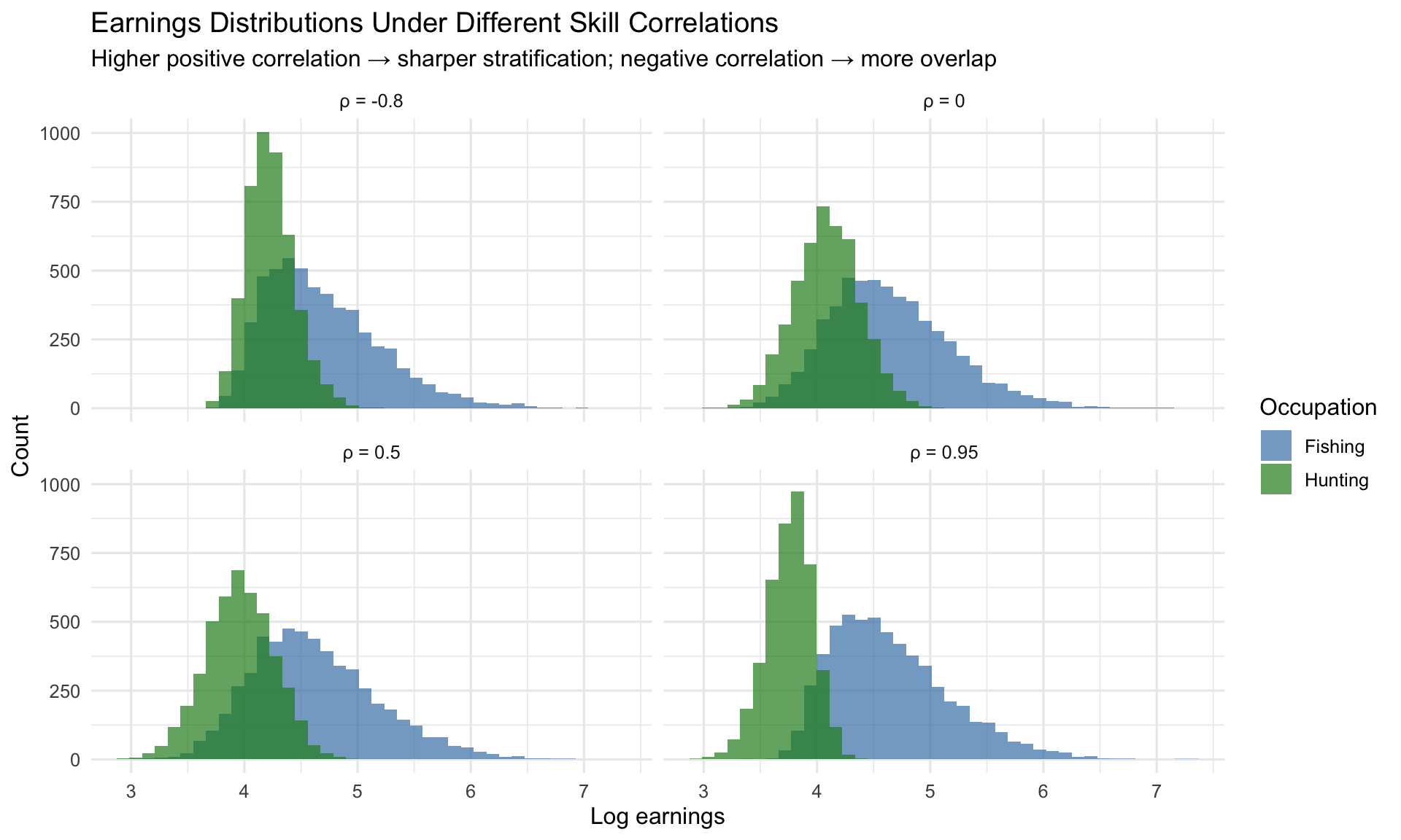

Figure 7: How correlation shapes the earnings distribution

---

Section IV: Multiple Occupations

Roy extends the model to a more complex economy.

The Sophisticated Township

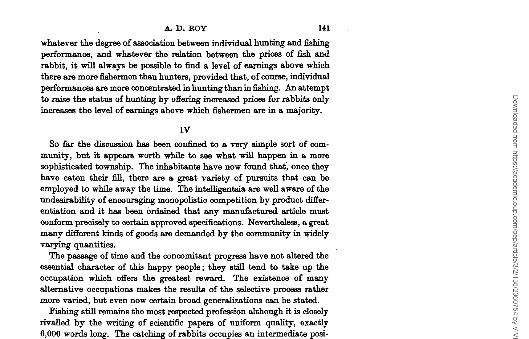
Now there are many occupations: fishing, writing scientific papers, hunting, chopping wood, carrying water. The hierarchy is determined by variance:

• Fishing: Least concentrated (highest variance) → highest status
• Science: Close second
• Hunting: Intermediate
• Wood-chopping: Low status
• Water-carrying: Most concentrated (lowest variance) → lowest status

---

Selection in Multiple Occupations

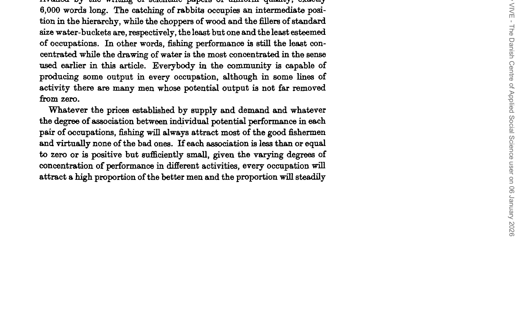
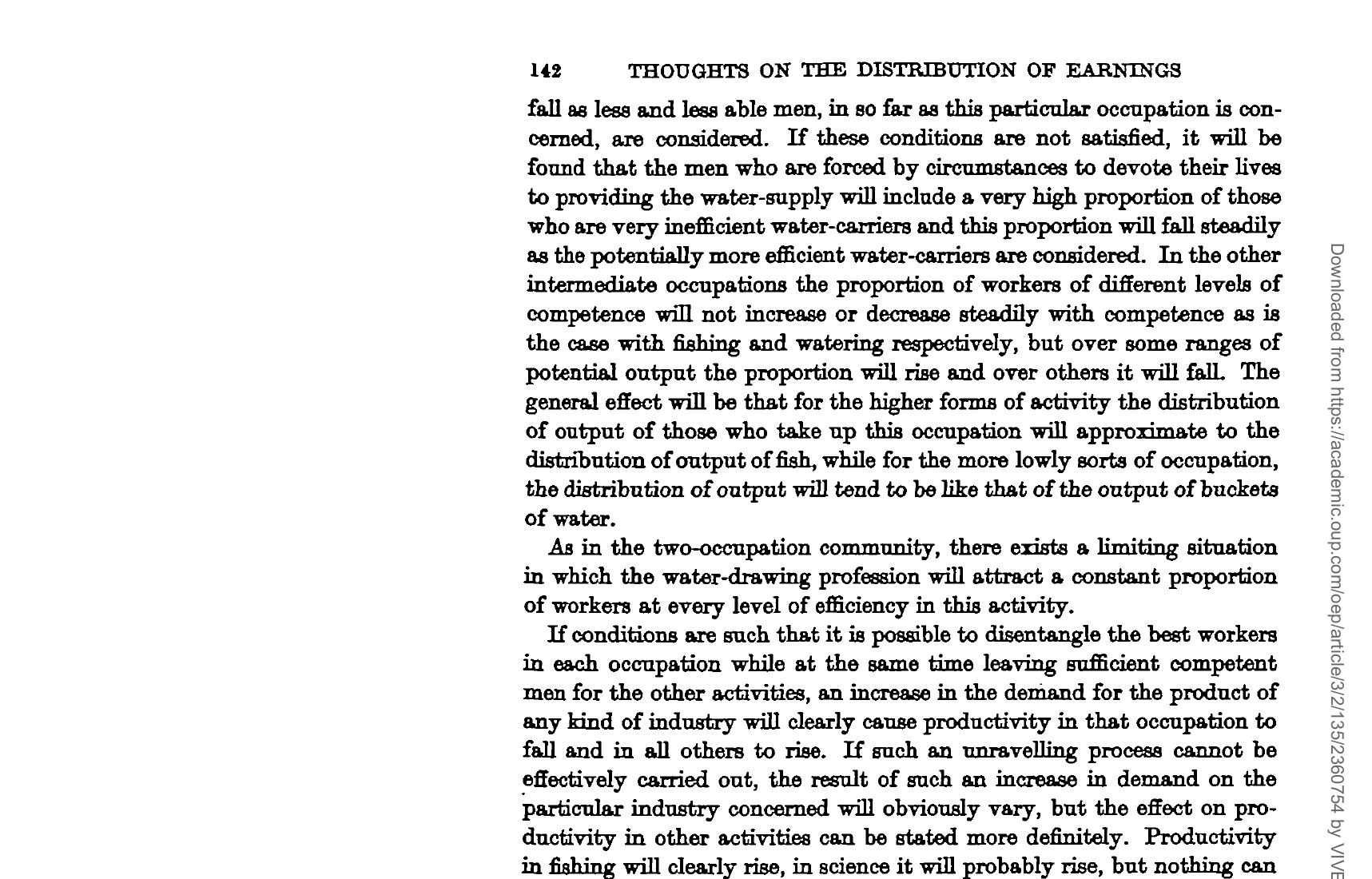
General principle: High-variance occupations attract the best workers in that skill. Low-variance occupations get “what’s left over” if skills are positively correlated.

---

Ay Bee’s Great-Grandson

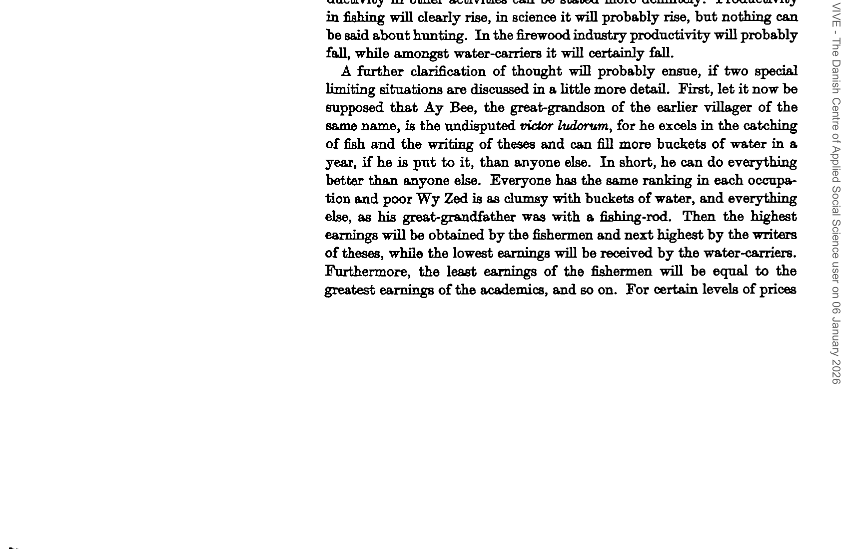
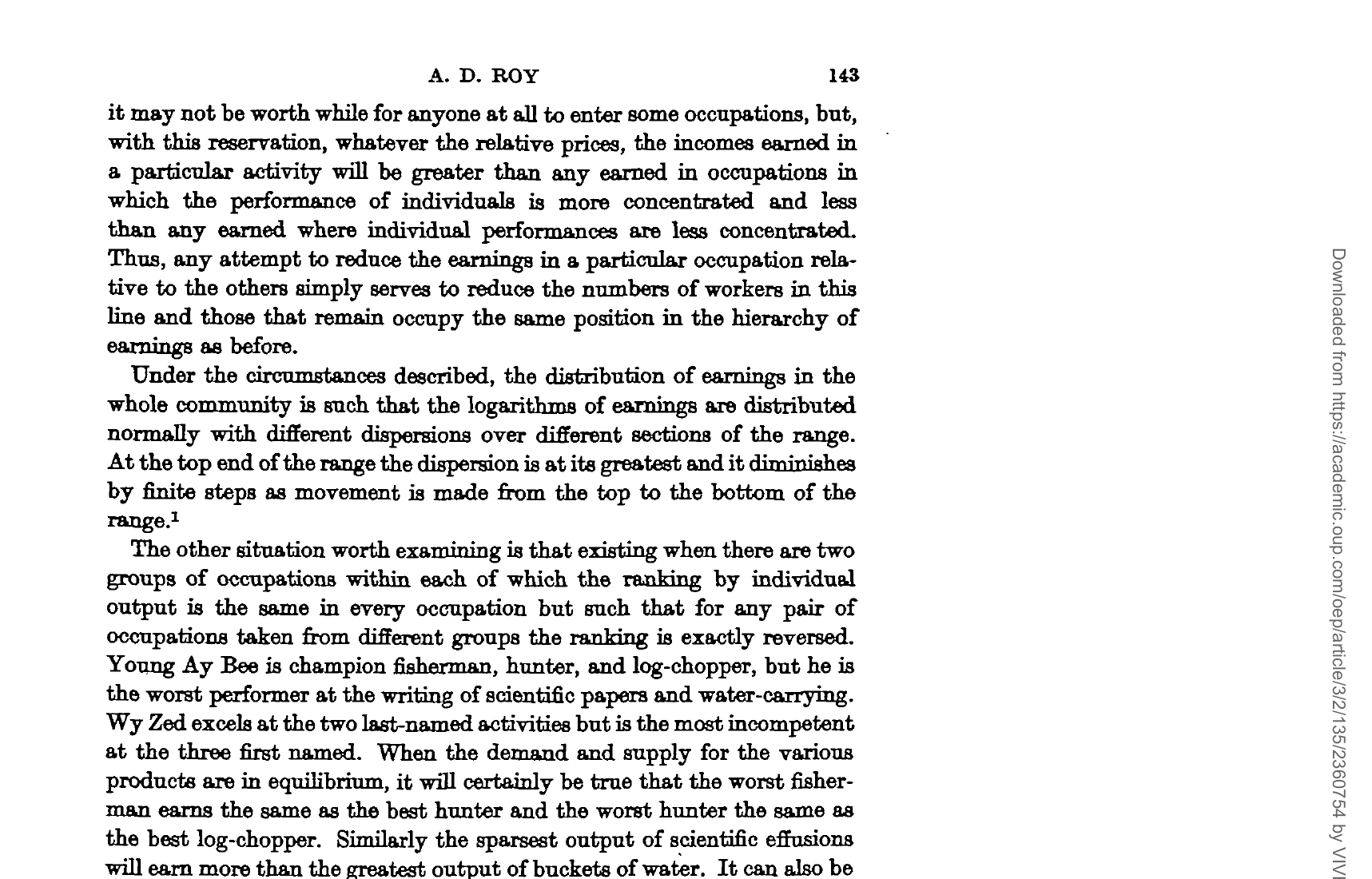
When one person (“Ay Bee”) is best at everything (ρ = 1 across all occupations), earnings form a strict hierarchy: all fishermen earn more than all scientists, who earn more than all hunters, etc.

Price manipulation can’t change this: Raising the price for water-carriers just drives workers out of that occupation—those who remain still earn less than everyone else.

---

The Two-Group Case

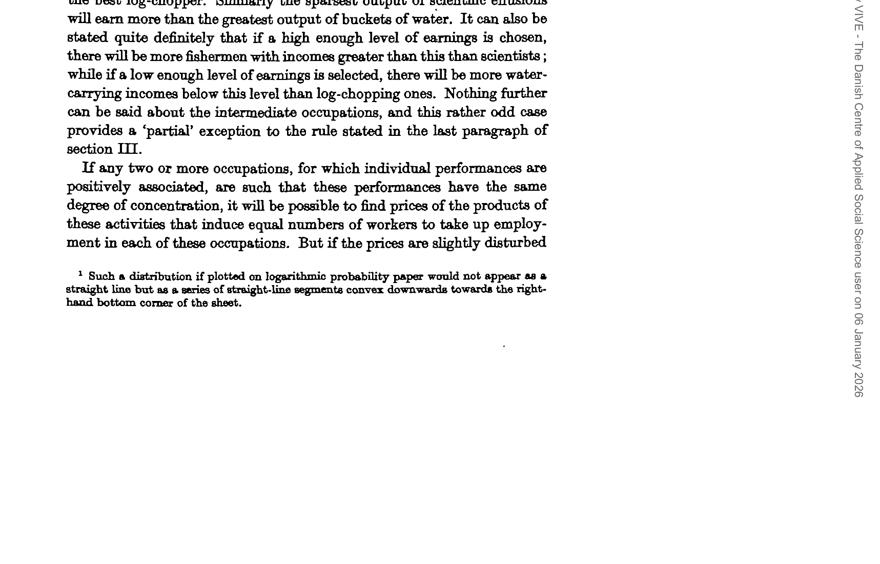
An interesting case: skills fall into two groups. “Ay Bee” excels at fishing, hunting, and wood-chopping, but is worst at science and water-carrying. “Wy Zed” is the reverse.

---

Section V: Relaxing Assumptions

Roy now considers how the model applies to reality.

Wages vs. Piece Rates

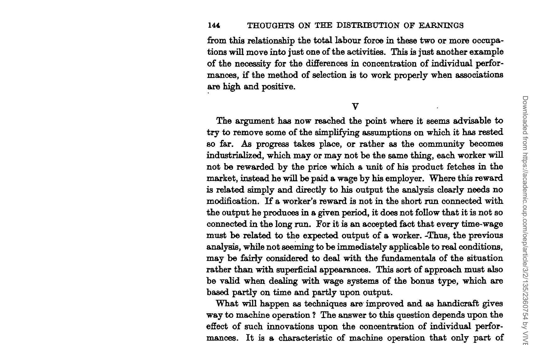
Even when workers are paid wages rather than piece rates, the analysis holds in the long run: wages must be related to expected output.

---

Technological Change

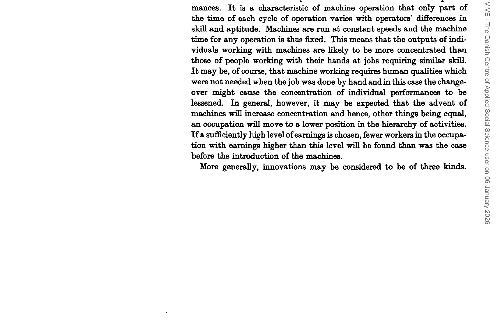
How machines affect occupational status:

Machines typically reduce variance by making the “machine time” constant—only the worker-dependent portion varies. This increases concentration.

R Simulation: Effect of Mechanization

Code

# Original vs mechanized hunting
village_original <- simulate_roy(n, rho = 0.5, sigma_h = 0.3, sigma_f = 0.8)
village_mechanized <- simulate_roy(n, rho = 0.5, sigma_h = 0.15, sigma_f = 0.8)

combined <- bind_rows(
  village_original |> mutate(scenario = "Original (σ_hunt = 0.3)"),
  village_mechanized |> mutate(scenario = "Mechanized (σ_hunt = 0.15)")
)

combined |>
  ggplot(aes(x = log(actual_earnings), fill = chosen)) +
  geom_histogram(bins = 40, alpha = 0.7, position = "identity") +
  facet_wrap(~scenario) +
  scale_fill_manual(values = c("Fishing" = "steelblue", "Hunting" = "forestgreen")) +
  labs(x = "Log earnings", y = "Count", fill = "Occupation",
       title = "Effect of Mechanization on Hunting",
       subtitle = "Lower variance → fewer hunters at top of earnings distribution") +
  theme_minimal(base_size = 12)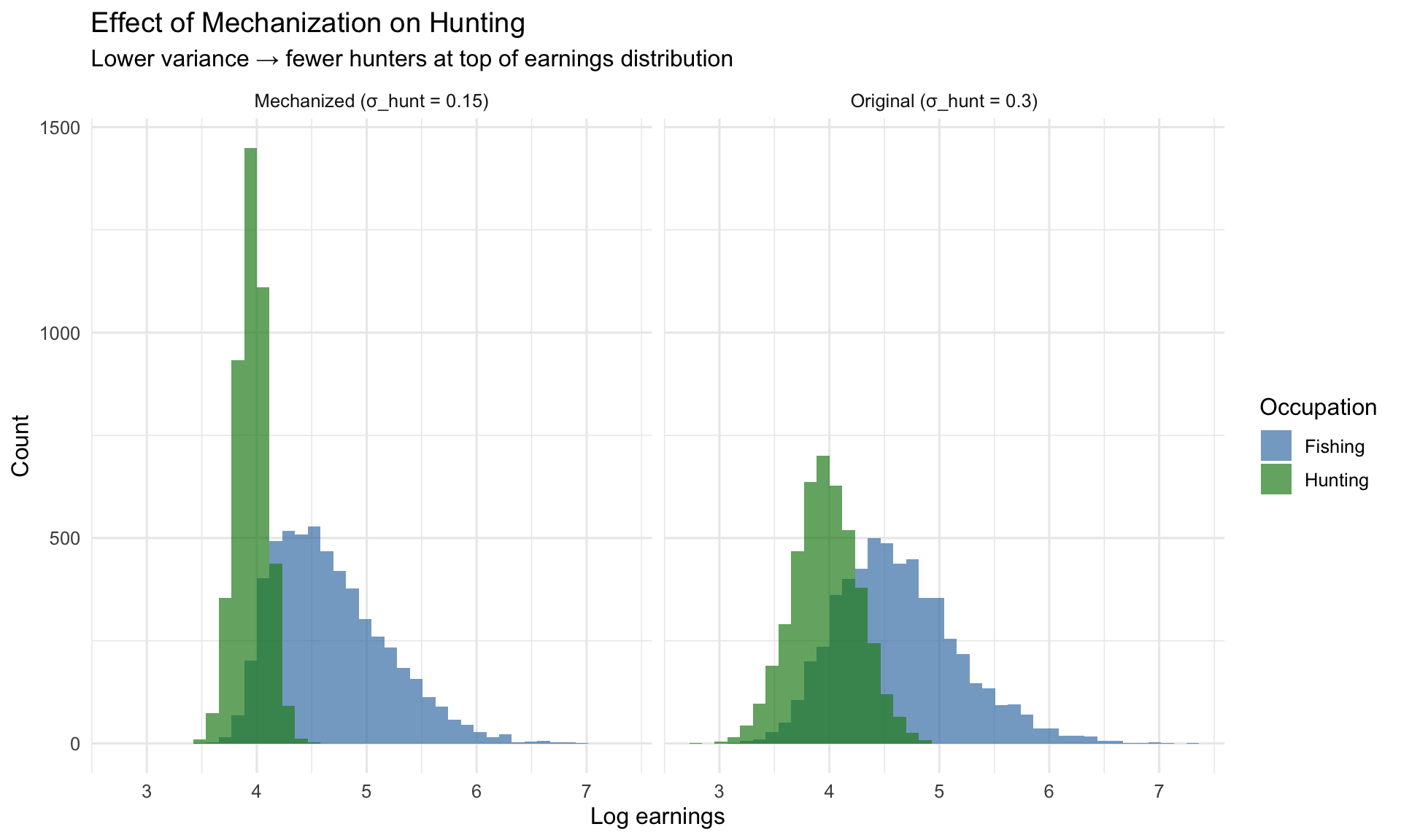

Figure 8: Mechanization increases concentration, lowering occupational status

---

Three Types of Innovation

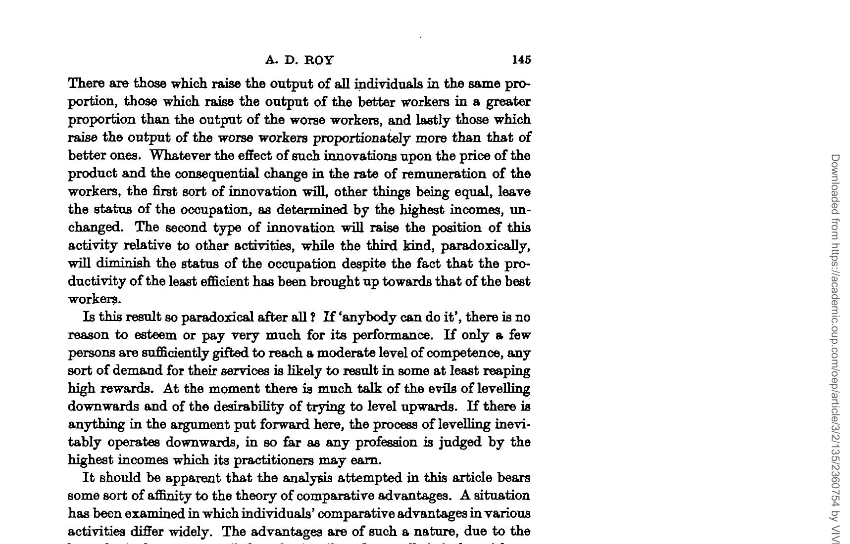
Roy identifies three types of technological change:

1. Proportional: Raises everyone’s output equally → status unchanged
2. Skill-biased: Helps better workers more → raises status
3. Skill-compressing: Helps worse workers more → lowers status

Paradox: “Levelling up” the worst workers actually lowers the occupation’s status!

---

“If Anybody Can Do It…”

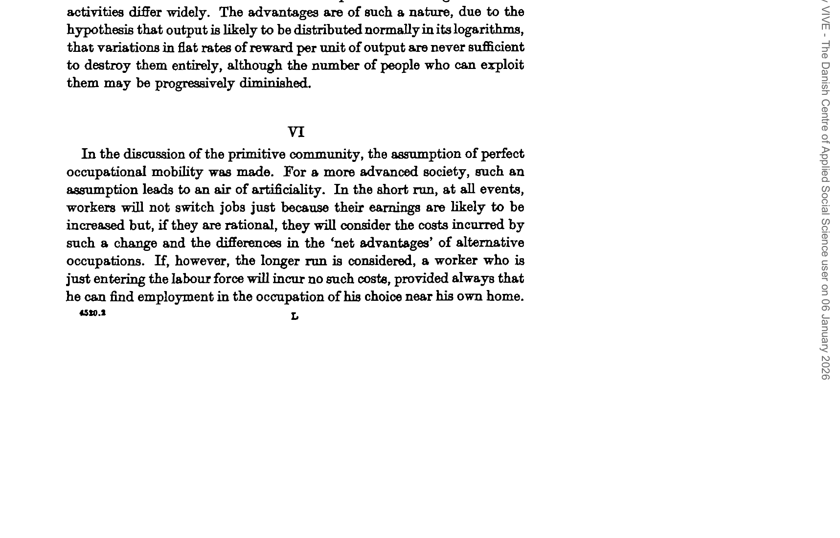
The key quote: “If ‘anybody can do it’, there is no reason to esteem or pay very much for its performance.”

Roy also notes the connection to comparative advantage: this is essentially a theory of individual comparative advantages in different activities.

R Simulation: Three Types of Innovation

Code

# Simulate three innovation types
# Type 1: Proportional (shift mean, keep variance)
# Type 2: Skill-biased (increase variance)
# Type 3: Skill-compressing (decrease variance)

village_base <- simulate_roy(n, rho = 0.5, sigma_h = 0.3)
village_skillbiased <- simulate_roy(n, rho = 0.5, sigma_h = 0.5)  # More variance
village_compressed <- simulate_roy(n, rho = 0.5, sigma_h = 0.15)  # Less variance

innovations <- bind_rows(
  village_base |> mutate(type = "1. Baseline (σ = 0.3)"),
  village_skillbiased |> mutate(type = "2. Skill-biased (σ = 0.5)"),
  village_compressed |> mutate(type = "3. Skill-compressed (σ = 0.15)")
)

# Show proportion of hunters at different earnings levels
innovations |>
  mutate(type = factor(type)) |>
  ggplot(aes(x = log(actual_earnings), fill = chosen)) +
  geom_histogram(bins = 40, alpha = 0.7, position = "identity") +
  facet_wrap(~type, ncol = 1) +
  scale_fill_manual(values = c("Fishing" = "steelblue", "Hunting" = "forestgreen")) +
  labs(x = "Log earnings", y = "Count", fill = "Occupation",
       title = "Three Types of Innovation in Hunting",
       subtitle = "Skill-biased raises hunting's status; skill-compressing lowers it") +
  theme_minimal(base_size = 12)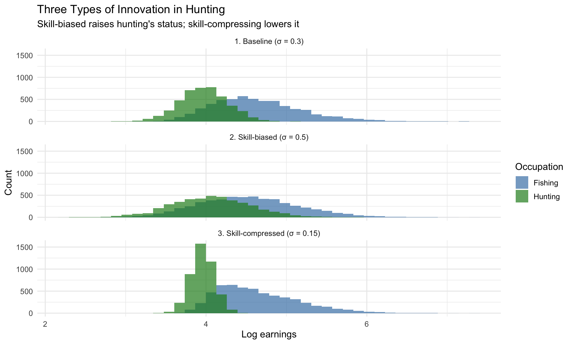

Figure 9: How different innovations affect occupational status

---

Section VI: Mobility Costs

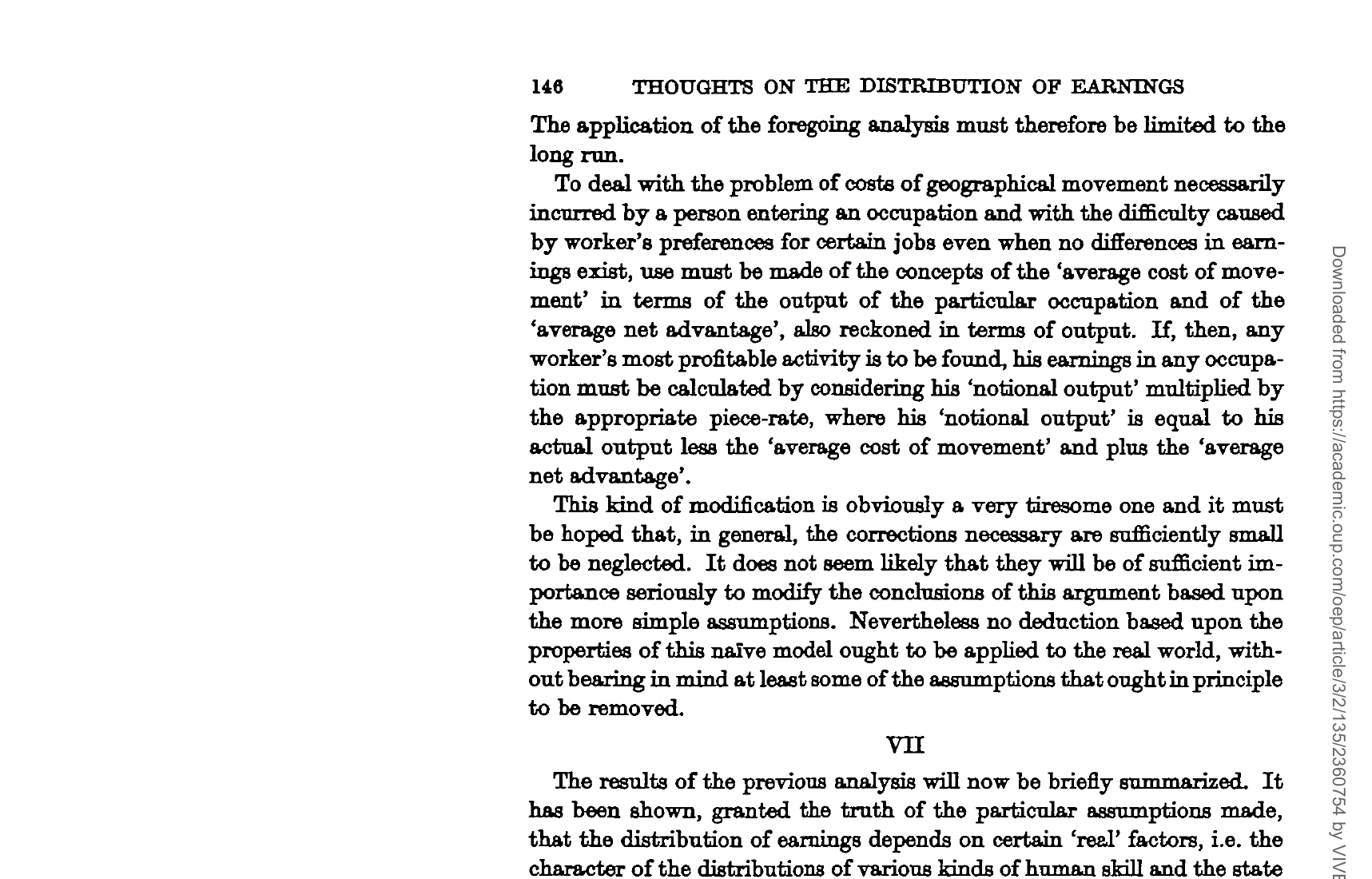
Roy acknowledges that in reality:

• Workers face costs to switch occupations
• Workers have preferences beyond just earnings
• Short-run mobility is limited

These can be incorporated as “notional output” adjustments, but Roy hopes they’re small enough to ignore.

---

Section VII: Summary

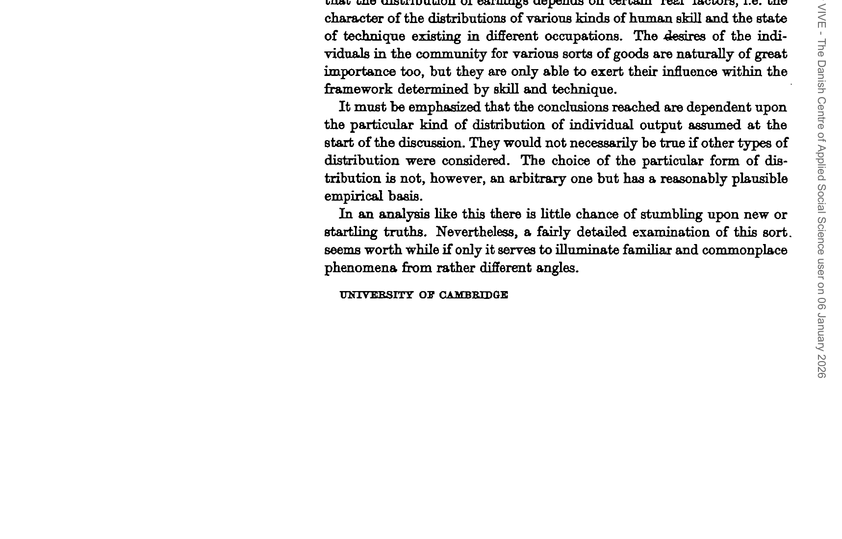
Roy’s conclusions:

1. The distribution of earnings depends on “real” factors: the distribution of human skills and the state of technology

2. Consumer preferences matter, but only within the framework set by skills and technology

3. The analysis depends on the log-normal assumption, which has empirical support

4. The model illuminates “familiar and commonplace phenomena from rather different angles”

---

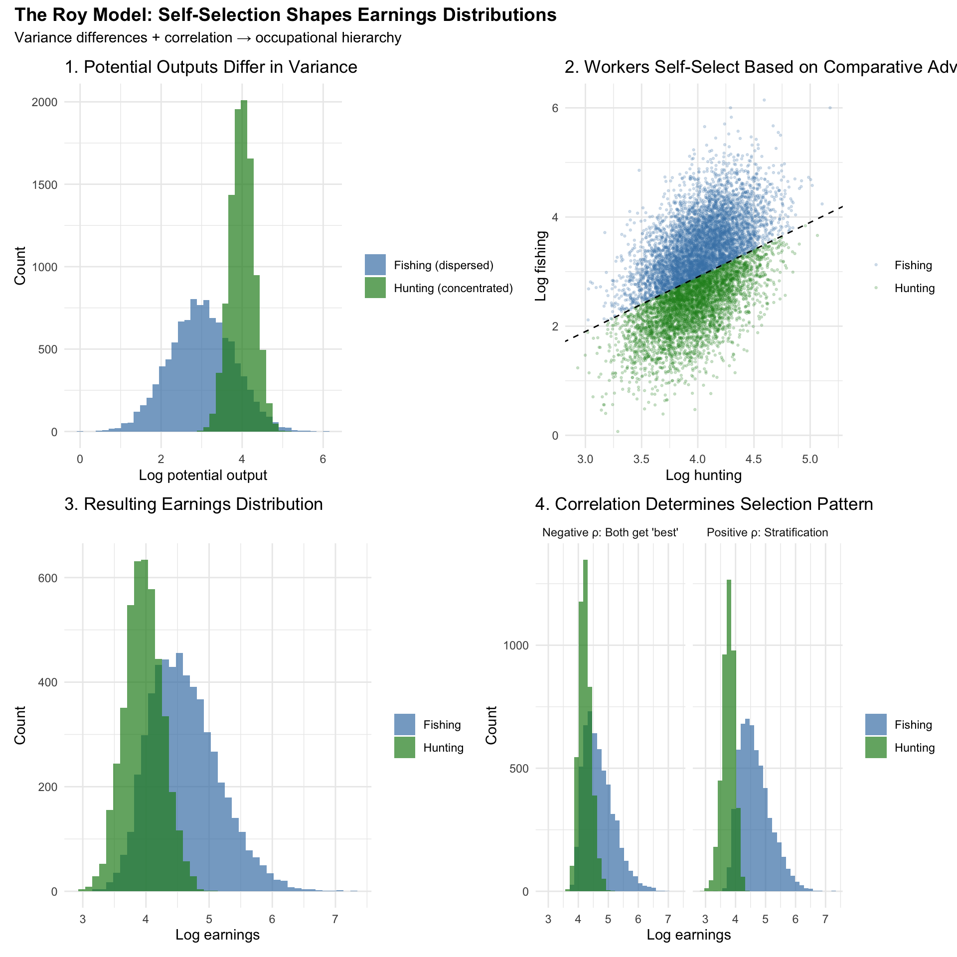
Final Summary: The Roy Model in Pictures

Code

# Create a comprehensive summary visualization
set.seed(1951)

# Panel 1: The two distributions
p1 <- village |>
  pivot_longer(cols = c(log_hunt, log_fish), names_to = "occ", values_to = "log_out") |>
  mutate(occ = if_else(occ == "log_hunt", "Hunting (concentrated)", "Fishing (dispersed)")) |>
  ggplot(aes(x = log_out, fill = occ)) +
  geom_histogram(bins = 40, alpha = 0.7, position = "identity") +
  scale_fill_manual(values = c("Hunting (concentrated)" = "forestgreen",
                                "Fishing (dispersed)" = "steelblue")) +
  labs(x = "Log potential output", y = "Count", fill = "",
       title = "1. Potential Outputs Differ in Variance") +
  theme_minimal(base_size = 11)

# Panel 2: Selection
p2 <- ggplot(village, aes(x = log_hunt, y = log_fish, color = chosen)) +
  geom_point(alpha = 0.2, size = 0.5) +
  geom_abline(intercept = log(1/3), slope = 1, linetype = "dashed") +
  scale_color_manual(values = c("Fishing" = "steelblue", "Hunting" = "forestgreen")) +
  labs(x = "Log hunting", y = "Log fishing", color = "",
       title = "2. Workers Self-Select Based on Comparative Advantage") +
  theme_minimal(base_size = 11)

# Panel 3: Resulting earnings
p3 <- ggplot(village, aes(x = log(actual_earnings), fill = chosen)) +
  geom_histogram(bins = 40, alpha = 0.7, position = "identity") +
  scale_fill_manual(values = c("Fishing" = "steelblue", "Hunting" = "forestgreen")) +
  labs(x = "Log earnings", y = "Count", fill = "",
       title = "3. Resulting Earnings Distribution") +
  theme_minimal(base_size = 11)

# Panel 4: Effect of correlation
p4 <- all_villages |>
  filter(rho %in% c(-0.8, 0.95)) |>
  mutate(rho_label = if_else(rho < 0, "Negative ρ: Both get 'best'",
                              "Positive ρ: Stratification")) |>
  ggplot(aes(x = log(actual_earnings), fill = chosen)) +
  geom_histogram(bins = 30, alpha = 0.7, position = "identity") +
  facet_wrap(~rho_label) +
  scale_fill_manual(values = c("Fishing" = "steelblue", "Hunting" = "forestgreen")) +
  labs(x = "Log earnings", y = "Count", fill = "",
       title = "4. Correlation Determines Selection Pattern") +
  theme_minimal(base_size = 11)

(p1 + p2) / (p3 + p4) +
  plot_annotation(
    title = "The Roy Model: Self-Selection Shapes Earnings Distributions",
    subtitle = "Variance differences + correlation → occupational hierarchy",
    theme = theme(plot.title = element_text(size = 14, face = "bold"))
  )

Figure 10: Summary: How the Roy Model works

---

Key Takeaways

1. Log-normal outputs arise from multiplicative random factors (health, skill, etc.)

2. Self-selection means observed distributions differ from potential distributions

3. Variance matters: High-variance occupations become “superior” because their top performers earn the most

4. Correlation matters: Positive correlation creates stratification; negative correlation creates specialization

5. Prices are superficial: They shift workers between occupations but can’t change the fundamental hierarchy

6. Technology shapes status: Innovations that compress variance lower an occupation’s status

This 1951 paper laid the foundation for modern selection models in labor economics, including the famous Heckman selection correction!

---

Session Info

Code

sessionInfo()

R version 4.4.2 (2024-10-31)
Platform: aarch64-apple-darwin20
Running under: macOS Sonoma 14.6.1

Matrix products: default
BLAS:   /Library/Frameworks/R.framework/Versions/4.4-arm64/Resources/lib/libRblas.0.dylib 
LAPACK: /Library/Frameworks/R.framework/Versions/4.4-arm64/Resources/lib/libRlapack.dylib;  LAPACK version 3.12.0

locale:
[1] en_US.UTF-8/en_US.UTF-8/en_US.UTF-8/C/en_US.UTF-8/en_US.UTF-8

time zone: Europe/Copenhagen
tzcode source: internal

attached base packages:
[1] stats     graphics  grDevices utils     datasets  methods   base     

other attached packages:
 [1] patchwork_1.3.0 MASS_7.3-61     lubridate_1.9.3 forcats_1.0.0  
 [5] stringr_1.5.1   dplyr_1.1.4     purrr_1.0.2     readr_2.1.5    
 [9] tidyr_1.3.1     tibble_3.3.0    ggplot2_3.5.2   tidyverse_2.0.0

loaded via a namespace (and not attached):
 [1] gtable_0.3.6       jsonlite_2.0.0     compiler_4.4.2     tidyselect_1.2.1  
 [5] scales_1.4.0       yaml_2.3.10        fastmap_1.2.0      R6_2.6.1          
 [9] labeling_0.4.3     generics_0.1.3     knitr_1.48         htmlwidgets_1.6.4 
[13] pillar_1.11.0      RColorBrewer_1.1-3 tzdb_0.4.0         rlang_1.1.6       
[17] stringi_1.8.4      xfun_0.49          timechange_0.3.0   cli_3.6.5         
[21] withr_3.0.2        magrittr_2.0.3     digest_0.6.37      grid_4.4.2        
[25] rstudioapi_0.17.1  hms_1.1.3          lifecycle_1.0.4    vctrs_0.6.5       
[29] evaluate_1.0.1     glue_1.8.0         farver_2.1.2       rmarkdown_2.29    
[33] tools_4.4.2        pkgconfig_2.0.3    htmltools_0.5.8.1